Static plotting for spatialdata#
In this notebook, we will explore how to use spatialdata-plot to generate static plots of various different technologies. When we load the spatialdata-plot library, this adds the .pl accessor to every SpatialData object, which gives us access to the plotting functions. Their logic is loosly inspired by the ggplot-library in R, in which one can chain multiple function calls, gradually building the final figure.
⚠️ Adjust the variable below to the data path on your specific workstation.
data_path = "../data/"
import spatialdata as sd
import spatialdata_plot as sdp
import matplotlib.pyplot as plt  # for multi-panel plots later
import scanpy as sc
import squidpy as sq

for p in [sd, sdp, sc, sq]:
    print(f"{p.__name__}: {p.__version__}")

sdata_visium = sd.read_zarr(data_path + "visium.zarr/")
spatialdata: 0.3.0
spatialdata_plot: 0.2.9
scanpy: 1.11.0
squidpy: 1.6.6.dev9+g78ed95c.d20250331
In particular, the library exposes the following functions:
We can chain the 4 render_xxx functions to gradually build up a figure, with a final call to show to then actually render out the function. In the following sections we will explore these functions further.
Simple function calls #
Let’s first focus on some Visium data from the previous notebook. As we can see below, it contains slots for Images, Shapes, and Tables.
sdata_visium
SpatialData object, with associated Zarr store: /Users/tim.treis/Documents/GitHub/202504_workshop_GSCN/notebooks/day_2/spatialdata/data/visium.zarr
├── Images
│     ├── 'CytAssist_FFPE_Protein_Expression_Human_Glioblastoma_hires_image': DataArray[cyx] (3, 2000, 1744)
│     └── 'CytAssist_FFPE_Protein_Expression_Human_Glioblastoma_lowres_image': DataArray[cyx] (3, 600, 523)
├── Shapes
│     └── 'CytAssist_FFPE_Protein_Expression_Human_Glioblastoma': GeoDataFrame shape: (5756, 2) (2D shapes)
└── Tables
      └── 'table': AnnData (5756, 18085)
with coordinate systems:
    ▸ 'downscaled_hires', with elements:
        CytAssist_FFPE_Protein_Expression_Human_Glioblastoma_hires_image (Images), CytAssist_FFPE_Protein_Expression_Human_Glioblastoma (Shapes)
    ▸ 'downscaled_lowres', with elements:
        CytAssist_FFPE_Protein_Expression_Human_Glioblastoma_lowres_image (Images), CytAssist_FFPE_Protein_Expression_Human_Glioblastoma (Shapes)
    ▸ 'global', with elements:
        CytAssist_FFPE_Protein_Expression_Human_Glioblastoma_hires_image (Images), CytAssist_FFPE_Protein_Expression_Human_Glioblastoma_lowres_image (Images), CytAssist_FFPE_Protein_Expression_Human_Glioblastoma (Shapes)
Let’s first visualize the individual contained modalities separately. When rendering the images, we see that we get two plots. That’s because the SpatialData object contains two coordinate systems (downscaled_hires and downscaled_lowres) with images aligned to them. The global coordinate system doesn’t contain any, as visible above.
sdata_visium.pl.render_images().pl.show()
INFO     Rasterizing image for faster rendering.
INFO     Rasterizing image for faster rendering.

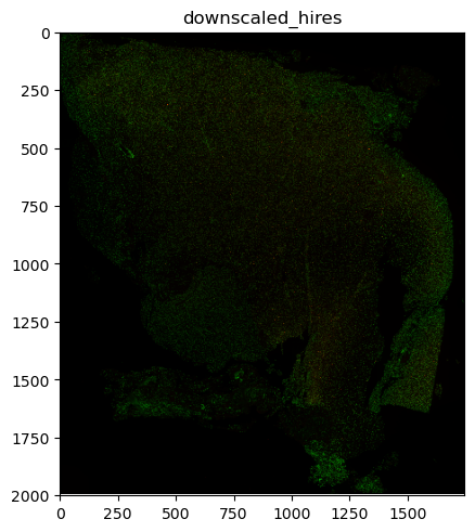
We can pass the name of a specific coordinate system to the pl.show() function to only render elements of that coordinate system.
sdata_visium.pl.render_images().pl.show(coordinate_systems="downscaled_hires")
INFO Rasterizing image for faster rendering.
The Visium technology works by detecting transcripts in specific circular caption locations (often referred to as “Visium spots”) on a slide. The circular capture locations are defined by the Shapes slot, which contains their coordinates. The Tables slot contains the actual transcript counts for each capture location. We can use the render_shapes function to overlay these circular locations onto our image.
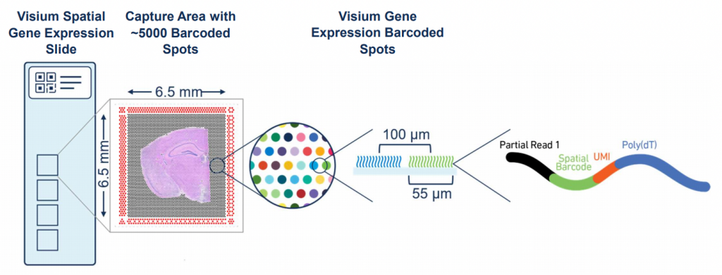
Image: The Visium Spatial Gene Expression Slide (https://www.10xgenomics.com/)
(
    sdata_visium.pl.render_images()
    .pl.render_shapes(fill_alpha=0.2)
    .pl.show("downscaled_hires", figsize=(8, 8))
)
INFO Rasterizing image for faster rendering.
Identify some genes with spatial patterns#
However, simply overlaying these locations doesn’t really contain much information. Ideally we want to investigate spatial trends in the gene expression data. For this we’re going to use Squidpy, another scverse package that contains several spatial analysis tools. We’ll use it to calculate the spatial autocorrelation of some genes, more specifically Moran’s I. This measure describes how homogenous a gene is expressed across a slide:
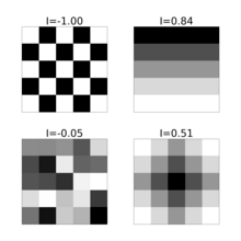
Image: https://en.wikipedia.org/wiki/Moran’s_I
adata_visium = sdata_visium.tables["table"]

sq.gr.spatial_neighbors(adata_visium)
sq.gr.spatial_autocorr(
    adata_visium,
    mode="moran",
    genes=adata_visium.var_names,
    n_perms=10,
    n_jobs=1,
)
/Users/tim.treis/anaconda3/envs/spatialdata-workshop/lib/python3.11/site-packages/scanpy/metrics/_common.py:73: UserWarning: 43 variables were constant, will return nan for these.
  warnings.warn(
print(adata_visium.uns["moranI"])
                   I  pval_norm  var_norm  pval_z_sim  pval_sim   var_sim  \
CST3        0.925848        0.0  0.000061         0.0  0.090909  0.000172
GFAP        0.907449        0.0  0.000061         0.0  0.090909  0.000117
IFI6        0.903449        0.0  0.000061         0.0  0.090909  0.000087
PTPRZ1      0.901717        0.0  0.000061         0.0  0.090909  0.000062
SPARC       0.900480        0.0  0.000061         0.0  0.090909  0.000048
...              ...        ...       ...         ...       ...       ...
NLGN4Y           NaN        NaN  0.000061         NaN  0.090909       NaN
AC007244.1       NaN        NaN  0.000061         NaN  0.090909       NaN
KDM5D            NaN        NaN  0.000061         NaN  0.090909       NaN
EIF1AY           NaN        NaN  0.000061         NaN  0.090909       NaN
DAZ2             NaN        NaN  0.000061         NaN  0.090909       NaN

            pval_norm_fdr_bh  pval_z_sim_fdr_bh  pval_sim_fdr_bh
CST3                     NaN                NaN         0.106628
GFAP                     NaN                NaN         0.106628
IFI6                     NaN                NaN         0.106628
PTPRZ1                   NaN                NaN         0.106628
SPARC                    NaN                NaN         0.106628
...                      ...                ...              ...
NLGN4Y                   NaN                NaN         0.106628
AC007244.1               NaN                NaN         0.106628
KDM5D                    NaN                NaN         0.106628
EIF1AY                   NaN                NaN         0.106628
DAZ2                     NaN                NaN         0.106628

[18085 rows x 9 columns]
print(adata_visium.uns["moranI"].head(3))
print(abs(adata_visium.uns["moranI"][~adata_visium.uns["moranI"]["I"].isna()]).tail(3))
             I  pval_norm  var_norm  pval_z_sim  pval_sim   var_sim  \
CST3  0.925848        0.0  0.000061         0.0  0.090909  0.000172
GFAP  0.907449        0.0  0.000061         0.0  0.090909  0.000117
IFI6  0.903449        0.0  0.000061         0.0  0.090909  0.000087

      pval_norm_fdr_bh  pval_z_sim_fdr_bh  pval_sim_fdr_bh
CST3               NaN                NaN         0.106628
GFAP               NaN                NaN         0.106628
IFI6               NaN                NaN         0.106628
                I  pval_norm  var_norm  pval_z_sim  pval_sim   var_sim  \
FAM81B   0.012231   0.061272  0.000061    0.003717  0.090909  0.000032
FOXD3    0.012730   0.053913  0.000061    0.004170  0.090909  0.000034
COLEC10  0.013522   0.043683  0.000061    0.000581  0.090909  0.000024

         pval_norm_fdr_bh  pval_z_sim_fdr_bh  pval_sim_fdr_bh
FAM81B                NaN                NaN         0.106628
FOXD3                 NaN                NaN         0.106628
COLEC10               NaN                NaN         0.106628
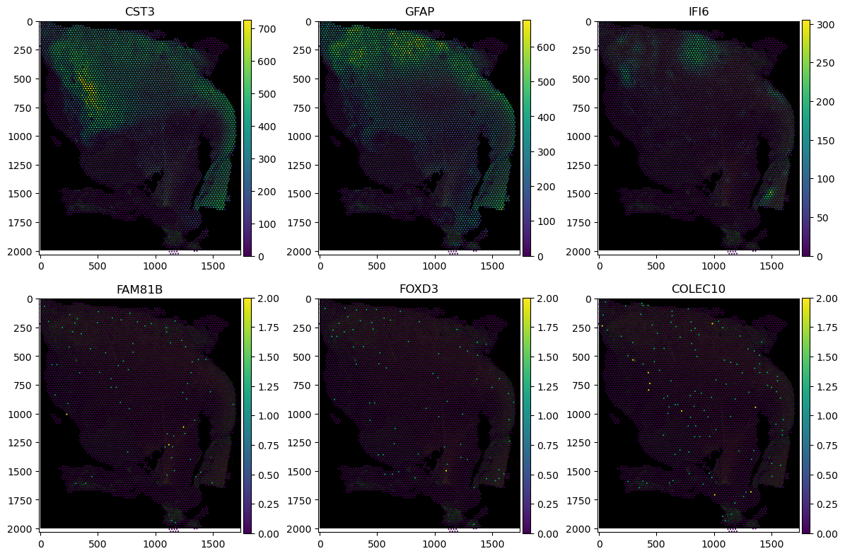
Let’s visualise the spatial expression of the 3 genes with the highest and lowest Moran’s I scores each. We’ll use classic matplotlib synthax to construct the multi-panel figure.
fig, axs = plt.subplots(2, 3, figsize=(12, 8))

for idx, gene in enumerate(["CST3", "GFAP", "IFI6", "FAM81B", "FOXD3", "COLEC10"]):
    (
        sdata_visium.pl.render_images()
        .pl.render_shapes(color=f"{gene}")
        .pl.show(
            "downscaled_hires",
            ax=axs[idx // 3, idx % 3],
            title=gene,
        )
    )

fig.tight_layout()
INFO Rasterizing image for faster rendering.
/Users/tim.treis/anaconda3/envs/spatialdata-workshop/lib/python3.11/site-packages/spatialdata/_core/_elements.py:105: UserWarning: Key `CytAssist_FFPE_Protein_Expression_Human_Glioblastoma` already exists. Overwriting it in-memory.
  self._check_key(key, self.keys(), self._shared_keys)
/Users/tim.treis/anaconda3/envs/spatialdata-workshop/lib/python3.11/site-packages/spatialdata/_core/_elements.py:125: UserWarning: Key `table` already exists. Overwriting it in-memory.
  self._check_key(key, self.keys(), self._shared_keys)
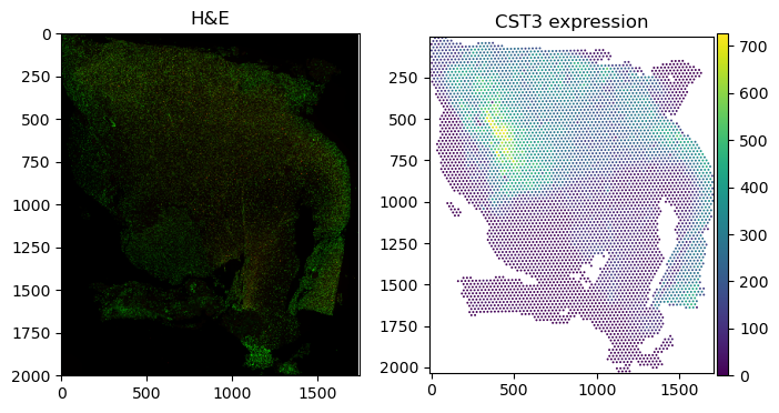
Generally, the spatialdata-plot library tries to be as flexible as possible, allowing for a wide range of different plotting options. However, this flexibility comes at the cost of some complexity. To limit the amount of permutations we have to account for in the codebase, we recommend a workflow in which one gradually builds up a figure on an ax object. If multiple similar plots are required, it is currently the easiest way, to manually assign them to their panels, for example like this:
fig, axs = plt.subplots(1, 2, figsize=(8, 4))

sdata_visium.pl.render_images().pl.show("downscaled_hires", ax=axs[0], title="H&E")

sdata_visium.pl.render_shapes(color="CST3").pl.show(
    "downscaled_hires", ax=axs[1], title="CST3 expression"
)
INFO Rasterizing image for faster rendering.
Clipping input data to the valid range for imshow with RGB data ([0..1] for floats or [0..255] for integers). Got range [0.0..1.0070922].
/Users/tim.treis/anaconda3/envs/spatialdata-workshop/lib/python3.11/site-packages/spatialdata/_core/_elements.py:105: UserWarning: Key `CytAssist_FFPE_Protein_Expression_Human_Glioblastoma` already exists. Overwriting it in-memory.
  self._check_key(key, self.keys(), self._shared_keys)
/Users/tim.treis/anaconda3/envs/spatialdata-workshop/lib/python3.11/site-packages/spatialdata/_core/_elements.py:125: UserWarning: Key `table` already exists. Overwriting it in-memory.
  self._check_key(key, self.keys(), self._shared_keys)
Other technology: Visum HD#
The true strength of the SpatialData ecosystems presents itself when considering the vast amount of different technology providers on the market. Usually, most of these would require a scientist to learn specialised analysis methods and data formats. However, with spatialdata, we can abstract away these differences and provide a unified interface to the data. This allows us to easily switch between different technologies, without having to change the analysis code.
As a practical example of this, let’s load some Visium HD data. This technology is somewhat similar to the regular Visium technology, but the spatial expression is no longer based on an hexagonal grid but instead on probes, arranged into a square grid, which can be aggregated into different resolutions. This allows the data to have sub-cellular precision. More details can be found in the publication.
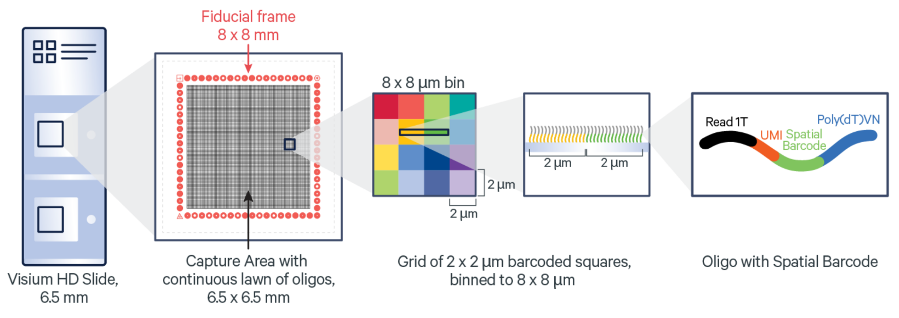
Image: https://www.10xgenomics.com/blog/your-introduction-to-visium-hd-spatial-biology-in-high-definition)
Similarly, to the regular Visium data, we can read and inspect the individual modalities contained in the data. We can see that the Visium HD data contains a lot more elements in the Shapes slot (351817 vs 5756) due to the increased precision.
sdata_visium_hd = sd.read_zarr(data_path + "visium_hd.zarr")
sdata_visium_hd
SpatialData object, with associated Zarr store: /Users/tim.treis/Documents/GitHub/202504_workshop_GSCN/notebooks/day_2/spatialdata/data/visium_hd.zarr
├── Images
│     ├── 'Visium_HD_Mouse_Small_Intestine_hires_image': DataArray[cyx] (3, 5575, 6000)
│     └── 'Visium_HD_Mouse_Small_Intestine_lowres_image': DataArray[cyx] (3, 558, 600)
├── Shapes
│     └── 'Visium_HD_Mouse_Small_Intestine_square_008um': GeoDataFrame shape: (351817, 1) (2D shapes)
└── Tables
      └── 'square_008um': AnnData (351817, 19059)
with coordinate systems:
    ▸ 'downscaled_hires', with elements:
        Visium_HD_Mouse_Small_Intestine_hires_image (Images), Visium_HD_Mouse_Small_Intestine_square_008um (Shapes)
    ▸ 'downscaled_lowres', with elements:
        Visium_HD_Mouse_Small_Intestine_lowres_image (Images), Visium_HD_Mouse_Small_Intestine_square_008um (Shapes)
    ▸ 'global', with elements:
        Visium_HD_Mouse_Small_Intestine_hires_image (Images), Visium_HD_Mouse_Small_Intestine_lowres_image (Images), Visium_HD_Mouse_Small_Intestine_square_008um (Shapes)
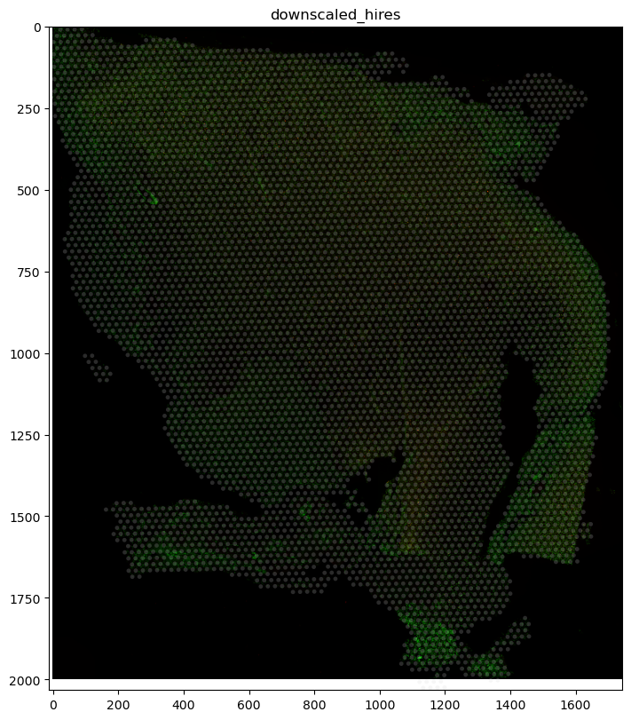
We can use the same synthax to visualise the individual modalities contained in the data.
sdata_visium_hd.pl.render_images().pl.show("downscaled_hires")
INFO Rasterizing image for faster rendering.
Clipping input data to the valid range for imshow with RGB data ([0..1] for floats or [0..255] for integers). Got range [-0.15..1.0].

We will use the .query.bounding_box() function to subset the data so that we can visually inspect the result easier. This function allows us to subset the data to a specific bounding box, which is defined by the top-left and bottom-right coordinates. This is useful when working with large datasets, as it allows us to only load the data that we’re interested in.
sdata_visium_hd_crop = sdata_visium_hd.query.bounding_box(
    axes=["x", "y"],
    min_coordinate=[4500, 0],
    max_coordinate=[6000, 1500],
    target_coordinate_system="downscaled_hires",
)
Let’s identify some genes with a high variance in expression across the slide for a quick proxy of Moran’s I and then visualise the spatial expression of these genes.
sdata_visium_hd_crop.tables["square_008um"].to_df().apply(
    lambda col: col.var(), axis=0
).sort_values()
Ptpn20           0.000000
Olfr718-ps1      0.000000
Spdye4b          0.000000
Zfp853           0.000000
Pou6f2           0.000000
                  ...
Iglc1           45.842403
Lyz1            50.397385
Defa21          58.193329
Igha           189.171158
Igkc           215.507874
Length: 19059, dtype: float32
sdata_visium_hd_crop.pl.render_shapes(color="Igha", method="matplotlib").pl.show(
    "downscaled_hires", figsize=(10, 10)
)
/Users/tim.treis/anaconda3/envs/spatialdata-workshop/lib/python3.11/site-packages/spatialdata/_core/_elements.py:105: UserWarning: Key `Visium_HD_Mouse_Small_Intestine_square_008um` already exists. Overwriting it in-memory.
  self._check_key(key, self.keys(), self._shared_keys)
/Users/tim.treis/anaconda3/envs/spatialdata-workshop/lib/python3.11/site-packages/spatialdata/_core/_elements.py:125: UserWarning: Key `square_008um` already exists. Overwriting it in-memory.
  self._check_key(key, self.keys(), self._shared_keys)
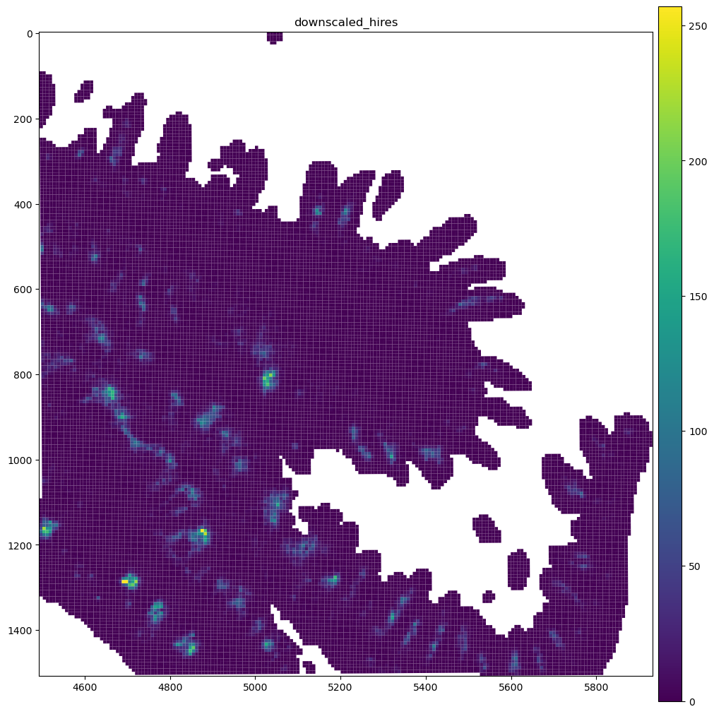
We can see that these bins are continous, so when overlaying the expression over an image, we would no longer see the image. To counter this, we will modify the colormap we’ll use so that true 0s in the expression matrix are shown fully transparent. The spatialdata-plot library provides a helper function for this.
from spatialdata_plot.pl.utils import set_zero_in_cmap_to_transparent

cmap = set_zero_in_cmap_to_transparent(plt.cm.viridis)
cmap

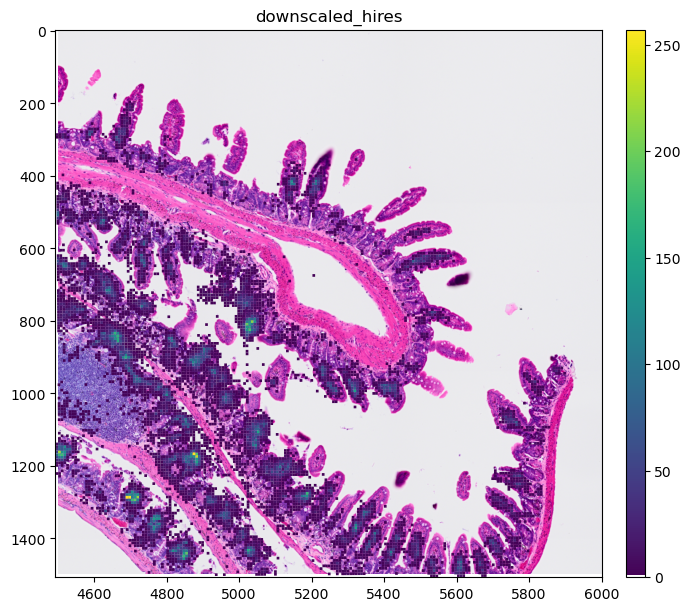
We can now use this cmap to visualise the spatial expression of the genes. We see that the gene is only expressed in certain areas of the slide.
sdata_visium_hd_crop.pl.render_images().pl.render_shapes(
    color="Igha", method="matplotlib", cmap=cmap
).pl.show("downscaled_hires", figsize=(8, 6))
Clipping input data to the valid range for imshow with RGB data ([0..1] for floats or [0..255] for integers). Got range [-0.16513762..1.0].
/Users/tim.treis/anaconda3/envs/spatialdata-workshop/lib/python3.11/site-packages/spatialdata/_core/_elements.py:105: UserWarning: Key `Visium_HD_Mouse_Small_Intestine_square_008um` already exists. Overwriting it in-memory.
  self._check_key(key, self.keys(), self._shared_keys)
/Users/tim.treis/anaconda3/envs/spatialdata-workshop/lib/python3.11/site-packages/spatialdata/_core/_elements.py:125: UserWarning: Key `square_008um` already exists. Overwriting it in-memory.
  self._check_key(key, self.keys(), self._shared_keys)
Some operations, such as plotting, can be accelerated by representing the Visium HD bins as pixels of an image. The function rasterize_bins() can be used for this; for its usage please refer to the Visium HD notebook from the documentation.
Other technology: Xenium#
Similar to Visium HD, the Xenium technology is a spatial transcriptomics technology that allows for sub-cellular precision. The main difference is that the transcripts here are never binned and are localised with (theoretically) arbitrary precision. This allows for a much higher resolution of the data, but also makes the data much more sparse.
sdata_xenium = sd.read_zarr(data_path + "xenium.zarr")
sdata_xenium
/Users/tim.treis/anaconda3/envs/spatialdata-workshop/lib/python3.11/site-packages/anndata/_core/aligned_df.py:68: ImplicitModificationWarning: Transforming to str index.
  warnings.warn("Transforming to str index.", ImplicitModificationWarning)
SpatialData object, with associated Zarr store: /Users/tim.treis/Documents/GitHub/202504_workshop_GSCN/notebooks/day_2/spatialdata/data/xenium.zarr
├── Images
│     ├── 'he_image': DataTree[cyx] (3, 5636, 1448), (3, 2818, 724), (3, 1409, 362), (3, 704, 181), (3, 352, 90)
│     └── 'morphology_focus': DataTree[cyx] (1, 17098, 51187), (1, 8549, 25593), (1, 4274, 12796), (1, 2137, 6398), (1, 1068, 3199)
├── Labels
│     ├── 'cell_labels': DataTree[yx] (17098, 51187), (8549, 25593), (4274, 12796), (2137, 6398), (1068, 3199)
│     └── 'nucleus_labels': DataTree[yx] (17098, 51187), (8549, 25593), (4274, 12796), (2137, 6398), (1068, 3199)
├── Points
│     └── 'transcripts': DataFrame with shape: (<Delayed>, 11) (3D points)
├── Shapes
│     ├── 'cell_boundaries': GeoDataFrame shape: (162254, 1) (2D shapes)
│     ├── 'cell_circles': GeoDataFrame shape: (162254, 2) (2D shapes)
│     └── 'nucleus_boundaries': GeoDataFrame shape: (156628, 1) (2D shapes)
└── Tables
      └── 'table': AnnData (162254, 377)
with coordinate systems:
    ▸ 'global', with elements:
        he_image (Images), morphology_focus (Images), cell_labels (Labels), nucleus_labels (Labels), transcripts (Points), cell_boundaries (Shapes), cell_circles (Shapes), nucleus_boundaries (Shapes)
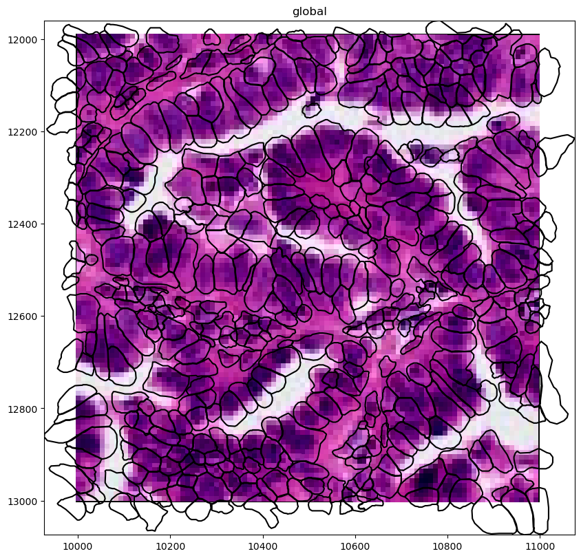
We will explore this data more in detail in of our next notebooks but will use the image here to show some benefits of using the spatialdata-plot library with large data.
crop = lambda sdata: sdata.query.bounding_box(
    min_coordinate=[10000, 12000],
    max_coordinate=[11000, 13000],
    axes=("x", "y"),
    target_coordinate_system="global",
)

(
    crop(sdata_xenium)
    .pl.render_images("he_image")
    .pl.render_shapes("cell_boundaries", fill_alpha=0, outline_alpha=1)
    .pl.show("global", figsize=(16, 8))
)
/Users/tim.treis/anaconda3/envs/spatialdata-workshop/lib/python3.11/functools.py:909: UserWarning: The object has `points` element. Depending on the number of points, querying MAY suffer from performance issues. Please consider filtering the object before calling this function by calling the `subset()` method of `SpatialData`.
  return dispatch(args[0].__class__)(*args, **kw)
Clipping input data to the valid range for imshow with RGB data ([0..1] for floats or [0..255] for integers). Got range [-0.275..1.0].
# the xenium gene expression in annotating the cell circles, let's switch the annoation to the cell boundaries (polygons)
sdata_xenium.tables["table"].obs["region"] = "cell_boundaries"
sdata_xenium.set_table_annotates_spatialelement("table", region="cell_boundaries")
/Users/tim.treis/anaconda3/envs/spatialdata-workshop/lib/python3.11/site-packages/spatialdata/_core/spatialdata.py:511: UserWarning: Converting `region_key: region` to categorical dtype.
  convert_region_column_to_categorical(table)
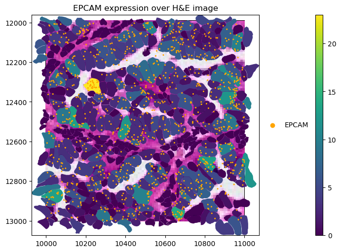
gene_name = "EPCAM"

crop(sdata_xenium).pl.render_images("he_image").pl.render_shapes(
    "cell_boundaries",
    color=gene_name,
).pl.render_points(
    "transcripts",
    color="feature_name",
    groups=gene_name,
    palette="orange",
).pl.show(
    title=f"{gene_name} expression over H&E image",
    coordinate_systems="global",
    figsize=(10, 5),
)
/Users/tim.treis/anaconda3/envs/spatialdata-workshop/lib/python3.11/functools.py:909: UserWarning: The object has `points` element. Depending on the number of points, querying MAY suffer from performance issues. Please consider filtering the object before calling this function by calling the `subset()` method of `SpatialData`.
  return dispatch(args[0].__class__)(*args, **kw)
Clipping input data to the valid range for imshow with RGB data ([0..1] for floats or [0..255] for integers). Got range [-0.275..1.0].
INFO input has more than 103 categories. Uniform 'grey' color will be used for all categories.
/Users/tim.treis/anaconda3/envs/spatialdata-workshop/lib/python3.11/site-packages/spatialdata/_core/_elements.py:105: UserWarning: Key `cell_boundaries` already exists. Overwriting it in-memory.
  self._check_key(key, self.keys(), self._shared_keys)
/Users/tim.treis/anaconda3/envs/spatialdata-workshop/lib/python3.11/site-packages/spatialdata/_core/_elements.py:125: UserWarning: Key `table` already exists. Overwriting it in-memory.
  self._check_key(key, self.keys(), self._shared_keys)
/Users/tim.treis/anaconda3/envs/spatialdata-workshop/lib/python3.11/site-packages/anndata/_core/anndata.py:381: FutureWarning: The dtype argument is deprecated and will be removed in late 2024.
  warnings.warn(
/Users/tim.treis/anaconda3/envs/spatialdata-workshop/lib/python3.11/site-packages/anndata/_core/aligned_df.py:68: ImplicitModificationWarning: Transforming to str index.
  warnings.warn("Transforming to str index.", ImplicitModificationWarning)
/Users/tim.treis/anaconda3/envs/spatialdata-workshop/lib/python3.11/site-packages/spatialdata/_core/_elements.py:115: UserWarning: Key `transcripts` already exists. Overwriting it in-memory.
  self._check_key(key, self.keys(), self._shared_keys)
/Users/tim.treis/anaconda3/envs/spatialdata-workshop/lib/python3.11/site-packages/spatialdata_plot/pl/utils.py:771: FutureWarning: The default value of 'ignore' for the `na_action` parameter in pandas.Categorical.map is deprecated and will be changed to 'None' in a future version. Please set na_action to the desired value to avoid seeing this warning
  color_vector = color_source_vector.map(color_mapping)
/Users/tim.treis/anaconda3/envs/spatialdata-workshop/lib/python3.11/site-packages/spatialdata_plot/pl/render.py:669: UserWarning: No data for colormapping provided via 'c'. Parameters 'cmap', 'norm' will be ignored
  _cax = ax.scatter(