Introduction to SpatialData objects

⚠️ Adjust the variable below to the data path on your specific workstation.

data_path = "../data/"

Reading common raw data formats

The spatialdata-io library allows for reading common raw data formats. Here we show an example where 3 very different technologies from 10x Genomics are read into a general data structure, given by the SpatialData class. From the presentation you might remember that these are the elements that can be contained inside of a SpatialData object:

Visium

from spatialdata_io import visium, visium_hd, xenium

/Users/tim.treis/anaconda3/envs/spatialdata-workshop/lib/python3.11/site-packages/anndata/utils.py:434: FutureWarning: Importing read_text from `anndata` is deprecated. Import anndata.io.read_text instead.
  warnings.warn(msg, FutureWarning)

sdata_visium = visium(data_path + "visium_2.1.0_2_io_subset")

INFO     reading                                                                                                   
         ../data/visium_2.1.0_2_io_subset/CytAssist_FFPE_Protein_Expression_Human_Glioblastoma_filtered_feature_bc_
         matrix.h5                                                                                                 

/Users/tim.treis/anaconda3/envs/spatialdata-workshop/lib/python3.11/site-packages/anndata/_core/anndata.py:1758: UserWarning: Variable names are not unique. To make them unique, call `.var_names_make_unique`.
  utils.warn_names_duplicates("var")
/Users/tim.treis/anaconda3/envs/spatialdata-workshop/lib/python3.11/site-packages/anndata/_core/anndata.py:1758: UserWarning: Variable names are not unique. To make them unique, call `.var_names_make_unique`.
  utils.warn_names_duplicates("var")
/Users/tim.treis/anaconda3/envs/spatialdata-workshop/lib/python3.11/site-packages/spatialdata/models/models.py:1053: UserWarning: Converting `region_key: region` to categorical dtype.
  return convert_region_column_to_categorical(adata)

The warning above indicates that the variable names (in this case, genes) in the provided data are not unique. It is essential that the variable names are unique to ensure the accuracy of several analysis steps, so we’ll use the AnnData API to make sure of that.

sdata_visium.tables["table"].var_names_make_unique()  # modifies in-place

Let’s have a look at the SpatialData object we just created:

sdata_visium

SpatialData object
├── Images
│     ├── 'CytAssist_FFPE_Protein_Expression_Human_Glioblastoma_hires_image': DataArray[cyx] (3, 2000, 1744)
│     └── 'CytAssist_FFPE_Protein_Expression_Human_Glioblastoma_lowres_image': DataArray[cyx] (3, 600, 523)
├── Shapes
│     └── 'CytAssist_FFPE_Protein_Expression_Human_Glioblastoma': GeoDataFrame shape: (5756, 2) (2D shapes)
└── Tables
      └── 'table': AnnData (5756, 18085)
with coordinate systems:
    ▸ 'downscaled_hires', with elements:
        CytAssist_FFPE_Protein_Expression_Human_Glioblastoma_hires_image (Images), CytAssist_FFPE_Protein_Expression_Human_Glioblastoma (Shapes)
    ▸ 'downscaled_lowres', with elements:
        CytAssist_FFPE_Protein_Expression_Human_Glioblastoma_lowres_image (Images), CytAssist_FFPE_Protein_Expression_Human_Glioblastoma (Shapes)
    ▸ 'global', with elements:
        CytAssist_FFPE_Protein_Expression_Human_Glioblastoma_hires_image (Images), CytAssist_FFPE_Protein_Expression_Human_Glioblastoma_lowres_image (Images), CytAssist_FFPE_Protein_Expression_Human_Glioblastoma (Shapes)

Visium HD

sdata_visium_hd = visium_hd("../data/visium_hd_3.0.0_io_subset")

sdata_visium_hd

/Users/tim.treis/anaconda3/envs/spatialdata-workshop/lib/python3.11/site-packages/anndata/_core/anndata.py:1758: UserWarning: Variable names are not unique. To make them unique, call `.var_names_make_unique`.
  utils.warn_names_duplicates("var")
/var/folders/qg/qgc908995g3fc8qtss2fsbhhxyxxj4/T/ipykernel_54847/2629054539.py:1: UserWarning: No full resolution image found. If incorrect, please specify the path in the `fullres_image_file` parameter when calling the `visium_hd` reader function.
  sdata_visium_hd = visium_hd("../data/visium_hd_3.0.0_io_subset")

SpatialData object
├── Images
│     ├── 'Visium_HD_Mouse_Small_Intestine_hires_image': DataArray[cyx] (3, 5575, 6000)
│     └── 'Visium_HD_Mouse_Small_Intestine_lowres_image': DataArray[cyx] (3, 558, 600)
├── Shapes
│     └── 'Visium_HD_Mouse_Small_Intestine_square_008um': GeoDataFrame shape: (351817, 1) (2D shapes)
└── Tables
      └── 'square_008um': AnnData (351817, 19059)
with coordinate systems:
    ▸ 'downscaled_hires', with elements:
        Visium_HD_Mouse_Small_Intestine_hires_image (Images), Visium_HD_Mouse_Small_Intestine_square_008um (Shapes)
    ▸ 'downscaled_lowres', with elements:
        Visium_HD_Mouse_Small_Intestine_lowres_image (Images), Visium_HD_Mouse_Small_Intestine_square_008um (Shapes)
    ▸ 'global', with elements:
        Visium_HD_Mouse_Small_Intestine_hires_image (Images), Visium_HD_Mouse_Small_Intestine_lowres_image (Images), Visium_HD_Mouse_Small_Intestine_square_008um (Shapes)

sdata_visium_hd.tables["square_008um"].var_names_make_unique()  # modifies in-place

Xenium

sdata_xenium = xenium("../data/xenium_2.0.0_io_subset", cells_as_circles=True)

sdata_xenium

INFO     reading ../data/xenium_2.0.0_io_subset/cell_feature_matrix.h5                                             

<TiffTag.fromfile> raised TiffFileError('<tifffile.TiffTag 270 @124> invalid value offset 414390846')

SpatialData object
├── Images
│     ├── 'he_image': DataTree[cyx] (3, 5636, 1448), (3, 2818, 724), (3, 1409, 362), (3, 704, 181), (3, 352, 90)
│     └── 'morphology_focus': DataTree[cyx] (1, 17098, 51187), (1, 8549, 25593), (1, 4274, 12796), (1, 2137, 6398), (1, 1068, 3199)
├── Labels
│     ├── 'cell_labels': DataTree[yx] (17098, 51187), (8549, 25593), (4274, 12796), (2137, 6398), (1068, 3199)
│     └── 'nucleus_labels': DataTree[yx] (17098, 51187), (8549, 25593), (4274, 12796), (2137, 6398), (1068, 3199)
├── Points
│     └── 'transcripts': DataFrame with shape: (<Delayed>, 11) (3D points)
├── Shapes
│     ├── 'cell_boundaries': GeoDataFrame shape: (162254, 1) (2D shapes)
│     ├── 'cell_circles': GeoDataFrame shape: (162254, 2) (2D shapes)
│     └── 'nucleus_boundaries': GeoDataFrame shape: (156628, 1) (2D shapes)
└── Tables
      └── 'table': AnnData (162254, 377)
with coordinate systems:
    ▸ 'global', with elements:
        he_image (Images), morphology_focus (Images), cell_labels (Labels), nucleus_labels (Labels), transcripts (Points), cell_boundaries (Shapes), cell_circles (Shapes), nucleus_boundaries (Shapes)

Representation of a multiscale image:

Saving to the SpatialData Zarr format

We introduce a storage format that extends the NGFF (Next Generation File Format) specification. The NGFF specification is implemented in the OME-Zarr disk format; the SpatialData Zarr format is an extension of OME-Zarr and will eventually converge to it.

Practically you can write the data as follows.

⚠️ Please uncomment the following cells with write() if this is the first time you run this notebook. They are commented because they make automated testing of the notebook easier (faster and no overwrite of files used by other notebooks).

sdata_visium.write(data_path + "visium.zarr", overwrite=True)

INFO     The Zarr backing store has been changed from None the new file path: ../data/visium.zarr                  

sdata_visium_hd.write(data_path + "visium_hd.zarr", overwrite=True)

INFO     The Zarr backing store has been changed from None the new file path: ../data/visium_hd.zarr               

sdata_xenium.write(data_path + "xenium.zarr", overwrite=True)

<TiffTag.fromfile> raised TiffFileError('<tifffile.TiffTag 270 @124> invalid value offset 414390846')

INFO     The Zarr backing store has been changed from None the new file path: ../data/xenium.zarr                  

Loading SpatialData from a disk-backed .zarr

Tip:

Given a SpatialData .zarr file, you can print its text representation from a terminal with:
python -m spatialdata peek data.zarr.

Saving to .zarr and re-reading the data is generally recommended when the data is large, since our storage format is optimized for dealing with large collections of images, geometries and annotations. For instance, if you save the data to Zarr and need to access a portion of an iamge, you will be able to read that portion without having to read the whole image.

# spatialdata-io is not needed in case your data is already in the SpatialData Zarr format

import spatialdata as sd

sdata_visium = sd.read_zarr(data_path + "visium.zarr")
sdata_visium_hd = sd.read_zarr(data_path + "visium_hd.zarr")
sdata_xenium = sd.read_zarr(data_path + "xenium.zarr")

/Users/tim.treis/anaconda3/envs/spatialdata-workshop/lib/python3.11/site-packages/anndata/_core/aligned_df.py:68: ImplicitModificationWarning: Transforming to str index.
  warnings.warn("Transforming to str index.", ImplicitModificationWarning)

Exploring the core slots of a SpatialData object

A SpatialData object is a container for images, labels, shapes, points and tables. Each of this object is denoted with the term element. We will use this term often.

For instance, we will use the term “Shapes element” to denote a geometric object (as we will see below, a dataframe) containing all the cells for a sample. We will not use the term “shapes element” to denote a single cell (a single cell will be a single row in our geometric dataframe).

The spatialdata library does not introduce specific types for storing the elements, and rather adopts standard classes from the imaging and geospatial Python community.

We use the following classes for storing the elements:

• single-scale images and labels elements are represented as xarray.DataArray objects.

• multi-scale images and labels elements are represented as datatree.DataTree objects.

• shapes elements are represented as geopandas.GeoDataFrame objects.

• points elements are represented as a lazy version of a pandas.DataFrame object; i.e. as dask.DataFrame objects.

• tables elements are represented as anndata.AnnData objects.

In particular:

• 2D/3D (cyx/czyx) multi-channel single-scale/multi-scale images (e.g. large H&E images)

• 2D/3D (yx/zyx) single-scale/multi-scale labels (e.g. segmentation masks)

• 2D/3D (xy/xyz) points (e.g. transcripts locations with gene id information)

• 2D (xy) shapes (e.g. cell/nucleus boundaries, anatomical annotatoins)

• tables (sparse/dense matrices/dataframes annotating the data).

We will give a quick overview of these classes here below; please refer to the respective documentations for a deeper introduction.

In the following examples *we will not manipulate or plot the elements using spatialdata code; we will just use standard geospatial libraries. This is to exemplify and remark how the data types we use are interoperable. Later we will show how spatialdata adds a layer of convenience on top of the existing geospatial ecosystem, by providing APIs that are implemented under the hood for all the geometric types.

Images and Labels (xarray.DataArray)

image = sdata_visium.images[
    "CytAssist_FFPE_Protein_Expression_Human_Glioblastoma_hires_image"
]
image

<xarray.DataArray 'image' (c: 3, y: 2000, x: 1744)> Size: 10MB
dask.array<from-zarr, shape=(3, 2000, 1744), dtype=uint8, chunksize=(3, 2000, 1744), chunktype=numpy.ndarray>
Coordinates:
  * c        (c) <U1 12B 'r' 'g' 'b'
  * y        (y) float64 16kB 0.5 1.5 2.5 3.5 ... 1.998e+03 1.998e+03 2e+03
  * x        (x) float64 14kB 0.5 1.5 2.5 3.5 ... 1.742e+03 1.742e+03 1.744e+03
Attributes:
    transform:  {'downscaled_hires': Identity , 'global': Scale (c, y, x)\n  ...

xarray.DataArray

'image'

• c: 3
• y: 2000
• x: 1744

• dask.array<chunksize=(3, 2000, 1744), meta=np.ndarray>

  Array Chunk Bytes 9.98 MiB 9.98 MiB Shape (3, 2000, 1744) (3, 2000, 1744) Dask graph 1 chunks in 2 graph layers Data type uint8 numpy.ndarray

• Coordinates: (3)
  • c
    (c)
    <U1
    'r' 'g' 'b'

    array(['r', 'g', 'b'], dtype='<U1')

  • y
    (y)
    float64
    0.5 1.5 2.5 ... 1.998e+03 2e+03

    array([5.0000e-01, 1.5000e+00, 2.5000e+00, ..., 1.9975e+03, 1.9985e+03,
           1.9995e+03])

  • x
    (x)
    float64
    0.5 1.5 2.5 ... 1.742e+03 1.744e+03

    array([5.0000e-01, 1.5000e+00, 2.5000e+00, ..., 1.7415e+03, 1.7425e+03,
           1.7435e+03])

• Indexes: (3)
  • c
    PandasIndex

    PandasIndex(Index(['r', 'g', 'b'], dtype='object', name='c'))

  • y
    PandasIndex

    PandasIndex(Index([   0.5,    1.5,    2.5,    3.5,    4.5,    5.5,    6.5,    7.5,    8.5,
              9.5,
           ...
           1990.5, 1991.5, 1992.5, 1993.5, 1994.5, 1995.5, 1996.5, 1997.5, 1998.5,
           1999.5],
          dtype='float64', name='y', length=2000))

  • x
    PandasIndex

    PandasIndex(Index([   0.5,    1.5,    2.5,    3.5,    4.5,    5.5,    6.5,    7.5,    8.5,
              9.5,
           ...
           1734.5, 1735.5, 1736.5, 1737.5, 1738.5, 1739.5, 1740.5, 1741.5, 1742.5,
           1743.5],
          dtype='float64', name='x', length=1744))

• Attributes: (1)

  transform :

  {'downscaled_hires': Identity , 'global': Scale (c, y, x) [ 1. 14.10099925 14.10099925]}

image.plot.imshow()

<matplotlib.image.AxesImage at 0x307e51ed0>

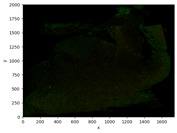
As you can see, the object is a regular xarray.DataArray object, a standard data structure in geospatial analysis. Therefore you can operate on the object with standard APIs or common external libraries (such as xarray-spatial.

For example:

import numpy as np

log_image = np.log1p(image).astype(np.float32)

log_image

<xarray.DataArray 'image' (c: 3, y: 2000, x: 1744)> Size: 42MB
dask.array<astype, shape=(3, 2000, 1744), dtype=float32, chunksize=(3, 2000, 1744), chunktype=numpy.ndarray>
Coordinates:
  * c        (c) <U1 12B 'r' 'g' 'b'
  * y        (y) float64 16kB 0.5 1.5 2.5 3.5 ... 1.998e+03 1.998e+03 2e+03
  * x        (x) float64 14kB 0.5 1.5 2.5 3.5 ... 1.742e+03 1.742e+03 1.744e+03
Attributes:
    transform:  {'CytAssist_FFPE_Protein_Expression_Human_Glioblastoma_downsc...

xarray.DataArray

'image'

• c: 3
• y: 2000
• x: 1744

• dask.array<chunksize=(3, 2000, 1744), meta=np.ndarray>

  Array Chunk Bytes 39.92 MiB 39.92 MiB Shape (3, 2000, 1744) (3, 2000, 1744) Dask graph 1 chunks in 7 graph layers Data type float32 numpy.ndarray

• Coordinates: (3)
  • c
    (c)
    <U1
    'r' 'g' 'b'

    long_name :

    c

    units :

    array(['r', 'g', 'b'], dtype='<U1')

  • y
    (y)
    float64
    0.5 1.5 2.5 ... 1.998e+03 2e+03

    array([5.0000e-01, 1.5000e+00, 2.5000e+00, ..., 1.9975e+03, 1.9985e+03,
           1.9995e+03])

  • x
    (x)
    float64
    0.5 1.5 2.5 ... 1.742e+03 1.744e+03

    array([5.0000e-01, 1.5000e+00, 2.5000e+00, ..., 1.7415e+03, 1.7425e+03,
           1.7435e+03])

• Indexes: (3)
  • c
    PandasIndex

    PandasIndex(Index(['r', 'g', 'b'], dtype='object', name='c'))

  • y
    PandasIndex

    PandasIndex(Index([   0.5,    1.5,    2.5,    3.5,    4.5,    5.5,    6.5,    7.5,    8.5,
              9.5,
           ...
           1990.5, 1991.5, 1992.5, 1993.5, 1994.5, 1995.5, 1996.5, 1997.5, 1998.5,
           1999.5],
          dtype='float64', name='y', length=2000))

  • x
    PandasIndex

    PandasIndex(Index([   0.5,    1.5,    2.5,    3.5,    4.5,    5.5,    6.5,    7.5,    8.5,
              9.5,
           ...
           1734.5, 1735.5, 1736.5, 1737.5, 1738.5, 1739.5, 1740.5, 1741.5, 1742.5,
           1743.5],
          dtype='float64', name='x', length=1744))

• Attributes: (1)

  transform :

  {'CytAssist_FFPE_Protein_Expression_Human_Glioblastoma_downscaled_hires': Identity , 'CytAssist_FFPE_Protein_Expression_Human_Glioblastoma': Scale (y, x) [14.10099925 14.10099925]}

As said, the image is a regular xarray.DataArray object, so we can for instance plot it using standard APIs.

The datatree.DataTree class (multiscale images and labels)

Multiscale images and labels are represented using the datatree.DataTree class.

We will use the Xenium dataset since the MERFISH ones does not contain any multiscale image.

sdata_xenium

SpatialData object
├── Images
│     ├── 'he_image': DataTree[cyx] (3, 5636, 1448), (3, 2818, 724), (3, 1409, 362), (3, 704, 181), (3, 352, 90)
│     └── 'morphology_focus': DataTree[cyx] (1, 17098, 51187), (1, 8549, 25593), (1, 4274, 12796), (1, 2137, 6398), (1, 1068, 3199)
├── Labels
│     ├── 'cell_labels': DataTree[yx] (17098, 51187), (8549, 25593), (4274, 12796), (2137, 6398), (1068, 3199)
│     └── 'nucleus_labels': DataTree[yx] (17098, 51187), (8549, 25593), (4274, 12796), (2137, 6398), (1068, 3199)
├── Points
│     └── 'transcripts': DataFrame with shape: (<Delayed>, 11) (3D points)
├── Shapes
│     ├── 'cell_boundaries': GeoDataFrame shape: (162254, 1) (2D shapes)
│     ├── 'cell_circles': GeoDataFrame shape: (162254, 2) (2D shapes)
│     └── 'nucleus_boundaries': GeoDataFrame shape: (156628, 1) (2D shapes)
└── Tables
      └── 'table': AnnData (162254, 377)
with coordinate systems:
    ▸ 'global', with elements:
        he_image (Images), morphology_focus (Images), cell_labels (Labels), nucleus_labels (Labels), transcripts (Points), cell_boundaries (Shapes), cell_circles (Shapes), nucleus_boundaries (Shapes)

Let’s load a labels object instead of an image. Images always have a channel c, labels never. What we will discuss for labels applies exaclty to images.

multiscale_labels = sdata_xenium["cell_labels"]
multiscale_labels

<xarray.DatasetView> Size: 0B
Dimensions:  ()
Data variables:
    *empty*

xarray.DataTree

• Groups: (5)
  <xarray.DatasetView> Size: 4GB
  Dimensions:  (y: 17098, x: 51187)
  Coordinates:
    * y        (y) float64 137kB 0.5 1.5 2.5 3.5 ... 1.71e+04 1.71e+04 1.71e+04
    * x        (x) float64 409kB 0.5 1.5 2.5 3.5 ... 5.118e+04 5.119e+04 5.119e+04
  Data variables:
      image    (y, x) uint32 4GB dask.array<chunksize=(4096, 4096), meta=np.ndarray>

  scale0

  • Groups: (0)
  • Dimensions:
    • y: 17098
    • x: 51187
  • Coordinates: (2)
    • y
      (y)
      float64
      0.5 1.5 2.5 ... 1.71e+04 1.71e+04

      array([5.00000e-01, 1.50000e+00, 2.50000e+00, ..., 1.70955e+04, 1.70965e+04,
             1.70975e+04])

    • x
      (x)
      float64
      0.5 1.5 2.5 ... 5.119e+04 5.119e+04

      array([5.00000e-01, 1.50000e+00, 2.50000e+00, ..., 5.11845e+04, 5.11855e+04,
             5.11865e+04])

  • Data variables: (1)
    • image
      (y, x)
      uint32
      dask.array<chunksize=(4096, 4096), meta=np.ndarray>

      transform :

      {'global': Identity }

      Array Chunk Bytes 3.26 GiB 64.00 MiB Shape (17098, 51187) (4096, 4096) Dask graph 65 chunks in 2 graph layers Data type uint32 numpy.ndarray

  • Attributes: (0)

  <xarray.DatasetView> Size: 875MB
  Dimensions:  (y: 8549, x: 25593)
  Coordinates:
    * y        (y) float64 68kB 1.0 3.0 5.0 7.0 ... 1.709e+04 1.71e+04 1.71e+04
    * x        (x) float64 205kB 1.0 3.0 5.0 7.0 ... 5.118e+04 5.118e+04 5.119e+04
  Data variables:
      image    (y, x) uint32 875MB dask.array<chunksize=(4096, 4096), meta=np.ndarray>

  scale1

  • Groups: (0)
  • Dimensions:
    • y: 8549
    • x: 25593
  • Coordinates: (2)
    • y
      (y)
      float64
      1.0 3.0 5.0 ... 1.71e+04 1.71e+04

      array([1.0000e+00, 3.0000e+00, 5.0000e+00, ..., 1.7093e+04, 1.7095e+04,
             1.7097e+04])

    • x
      (x)
      float64
      1.0 3.0 5.0 ... 5.118e+04 5.119e+04

      array([1.000020e+00, 3.000059e+00, 5.000098e+00, ..., 5.118200e+04,
             5.118400e+04, 5.118600e+04])

  • Data variables: (1)
    • image
      (y, x)
      uint32
      dask.array<chunksize=(4096, 4096), meta=np.ndarray>

      transform :

      {'global': Sequence Scale (y, x) [2. 2.00003907] Identity }

      Array Chunk Bytes 834.63 MiB 64.00 MiB Shape (8549, 25593) (4096, 4096) Dask graph 21 chunks in 1 graph layer Data type uint32 numpy.ndarray

  • Attributes: (0)

  <xarray.DatasetView> Size: 219MB
  Dimensions:  (y: 4274, x: 12796)
  Coordinates:
    * y        (y) float64 34kB 2.0 6.001 10.0 ... 1.709e+04 1.709e+04 1.71e+04
    * x        (x) float64 102kB 2.0 6.0 10.0 ... 5.118e+04 5.118e+04 5.118e+04
  Data variables:
      image    (y, x) uint32 219MB dask.array<chunksize=(4096, 4096), meta=np.ndarray>

  scale2

  • Groups: (0)
  • Dimensions:
    • y: 4274
    • x: 12796
  • Coordinates: (2)
    • y
      (y)
      float64
      2.0 6.001 ... 1.709e+04 1.71e+04

      array([2.000234e+00, 6.000702e+00, 1.000117e+01, ..., 1.708800e+04,
             1.709200e+04, 1.709600e+04])

    • x
      (x)
      float64
      2.0 6.0 ... 5.118e+04 5.118e+04

      array([2.000117e+00, 6.000352e+00, 1.000059e+01, ..., 5.117700e+04,
             5.118100e+04, 5.118500e+04])

  • Data variables: (1)
    • image
      (y, x)
      uint32
      dask.array<chunksize=(4096, 4096), meta=np.ndarray>

      transform :

      {'global': Sequence Scale (y, x) [4.00046795 4.00023445] Identity }

      Array Chunk Bytes 208.63 MiB 64.00 MiB Shape (4274, 12796) (4096, 4096) Dask graph 8 chunks in 1 graph layer Data type uint32 numpy.ndarray

  • Attributes: (0)

  <xarray.DatasetView> Size: 55MB
  Dimensions:  (y: 2137, x: 6398)
  Coordinates:
    * y        (y) float64 17kB 4.0 12.0 20.0 ... 1.708e+04 1.709e+04 1.709e+04
    * x        (x) float64 51kB 4.0 12.0 20.0 ... 5.117e+04 5.117e+04 5.118e+04
  Data variables:
      image    (y, x) uint32 55MB dask.array<chunksize=(2137, 4096), meta=np.ndarray>

  scale3

  • Groups: (0)
  • Dimensions:
    • y: 2137
    • x: 6398
  • Coordinates: (2)
    • y
      (y)
      float64
      4.0 12.0 ... 1.709e+04 1.709e+04

      array([4.000468e+00, 1.200140e+01, 2.000234e+01, ..., 1.707800e+04,
             1.708600e+04, 1.709400e+04])

    • x
      (x)
      float64
      4.0 12.0 ... 5.117e+04 5.118e+04

      array([4.000234e+00, 1.200070e+01, 2.000117e+01, ..., 5.116700e+04,
             5.117500e+04, 5.118300e+04])

  • Data variables: (1)
    • image
      (y, x)
      uint32
      dask.array<chunksize=(2137, 4096), meta=np.ndarray>

      transform :

      {'global': Sequence Scale (y, x) [8.00093589 8.0004689 ] Identity }

      Array Chunk Bytes 52.16 MiB 33.39 MiB Shape (2137, 6398) (2137, 4096) Dask graph 2 chunks in 1 graph layer Data type uint32 numpy.ndarray

  • Attributes: (0)

  <xarray.DatasetView> Size: 14MB
  Dimensions:  (y: 1068, x: 3199)
  Coordinates:
    * y        (y) float64 9kB 8.005 24.01 40.02 ... 1.706e+04 1.707e+04 1.709e+04
    * x        (x) float64 26kB 8.0 24.0 40.0 ... 5.115e+04 5.116e+04 5.118e+04
  Data variables:
      image    (y, x) uint32 14MB dask.array<chunksize=(1068, 3199), meta=np.ndarray>

  scale4

  • Groups: (0)
  • Dimensions:
    • y: 1068
    • x: 3199
  • Coordinates: (2)
    • y
      (y)
      float64
      8.005 24.01 ... 1.707e+04 1.709e+04

      array([8.004682e+00, 2.401404e+01, 4.002341e+01, ..., 1.705798e+04,
             1.707399e+04, 1.709000e+04])

    • x
      (x)
      float64
      8.0 24.0 ... 5.116e+04 5.118e+04

      array([8.000469e+00, 2.400141e+01, 4.000234e+01, ..., 5.114700e+04,
             5.116300e+04, 5.117900e+04])

  • Data variables: (1)
    • image
      (y, x)
      uint32
      dask.array<chunksize=(1068, 3199), meta=np.ndarray>

      transform :

      {'global': Sequence Scale (y, x) [16.0093633 16.00093779] Identity }

      Array Chunk Bytes 13.03 MiB 13.03 MiB Shape (1068, 3199) (1068, 3199) Dask graph 1 chunks in 1 graph layer Data type uint32 numpy.ndarray

  • Attributes: (0)

• Dimensions:
• Coordinates: (0)
• Inherited coordinates: (0)
• Data variables: (0)
• Attributes: (0)

The data tree has 5 groups, one for each scale of the multiscale labels. Each scale is a leaf of the tree (i.e. the tree doesn’t branch out again), also each scale could in principle contain multiple labels elements, but spatialdata requires for it to contain a single labels element. Let’s show an example on how to access the various scales and how to manipulate the object.

# show the scales
list(multiscale_labels.keys())

['scale0', 'scale1', 'scale2', 'scale3', 'scale4']

# access the scale 1
multiscale_labels["scale1"]

<xarray.DatasetView> Size: 875MB
Dimensions:  (y: 8549, x: 25593)
Coordinates:
  * y        (y) float64 68kB 1.0 3.0 5.0 7.0 ... 1.709e+04 1.71e+04 1.71e+04
  * x        (x) float64 205kB 1.0 3.0 5.0 7.0 ... 5.118e+04 5.118e+04 5.119e+04
Data variables:
    image    (y, x) uint32 875MB dask.array<chunksize=(4096, 4096), meta=np.ndarray>

xarray.DataTree

• Groups: (0)
• Dimensions:
  • y: 8549
  • x: 25593
• Coordinates: (2)
  • y
    (y)
    float64
    1.0 3.0 5.0 ... 1.71e+04 1.71e+04

    array([1.0000e+00, 3.0000e+00, 5.0000e+00, ..., 1.7093e+04, 1.7095e+04,
           1.7097e+04])

  • x
    (x)
    float64
    1.0 3.0 5.0 ... 5.118e+04 5.119e+04

    array([1.000020e+00, 3.000059e+00, 5.000098e+00, ..., 5.118200e+04,
           5.118400e+04, 5.118600e+04])

• Inherited coordinates: (0)
• Data variables: (1)
  • image
    (y, x)
    uint32
    dask.array<chunksize=(4096, 4096), meta=np.ndarray>

    transform :

    {'global': Sequence Scale (y, x) [2. 2.00003907] Identity }

    Array Chunk Bytes 834.63 MiB 64.00 MiB Shape (8549, 25593) (4096, 4096) Dask graph 21 chunks in 1 graph layer Data type uint32 numpy.ndarray

• Attributes: (0)

# this group contains a single-labels (as expected), called 'image'
# let's access such object
multiscale_labels["scale1"]["image"]

<xarray.DataArray 'image' (y: 8549, x: 25593)> Size: 875MB
dask.array<xarray-<this-array>, shape=(8549, 25593), dtype=uint32, chunksize=(4096, 4096), chunktype=numpy.ndarray>
Coordinates:
  * y        (y) float64 68kB 1.0 3.0 5.0 7.0 ... 1.709e+04 1.71e+04 1.71e+04
  * x        (x) float64 205kB 1.0 3.0 5.0 7.0 ... 5.118e+04 5.118e+04 5.119e+04
Attributes:
    transform:  {'global': Sequence \n    Scale (y, x)\n        [2.         2...

xarray.DataArray

'image'

• y: 8549
• x: 25593

• dask.array<chunksize=(4096, 4096), meta=np.ndarray>

  Array Chunk Bytes 834.63 MiB 64.00 MiB Shape (8549, 25593) (4096, 4096) Dask graph 21 chunks in 1 graph layer Data type uint32 numpy.ndarray

• Coordinates: (2)
  • y
    (y)
    float64
    1.0 3.0 5.0 ... 1.71e+04 1.71e+04

    array([1.0000e+00, 3.0000e+00, 5.0000e+00, ..., 1.7093e+04, 1.7095e+04,
           1.7097e+04])

  • x
    (x)
    float64
    1.0 3.0 5.0 ... 5.118e+04 5.119e+04

    array([1.000020e+00, 3.000059e+00, 5.000098e+00, ..., 5.118200e+04,
           5.118400e+04, 5.118600e+04])

• Indexes: (2)
  • y
    PandasIndex

    PandasIndex(Index([    1.0,     3.0,     5.0,     7.0,     9.0,    11.0,    13.0,    15.0,
              17.0,    19.0,
           ...
           17079.0, 17081.0, 17083.0, 17085.0, 17087.0, 17089.0, 17091.0, 17093.0,
           17095.0, 17097.0],
          dtype='float64', name='y', length=8549))

  • x
    PandasIndex

    PandasIndex(Index([1.0000195365920368, 3.0000586097761106,  5.000097682960184,
            7.000136756144258,  9.000175829328331, 11.000214902512404,
           13.000253975696479, 15.000293048880552, 17.000332122064627,
             19.0003711952487,
           ...
            51167.99962880475, 51169.999667877935, 51171.999706951116,
             51173.9997460243,  51175.99978509748,  51177.99982417067,
            51179.99986324385,  51181.99990231704,  51183.99994139022,
           51185.999980463406],
          dtype='float64', name='x', length=25593))

• Attributes: (1)

  transform :

  {'global': Sequence Scale (y, x) [2. 2.00003907] Identity }

Note how the labels is a xarray.DataArray object. So, as expected, a multiscale labels is a collection of single scale labels.

Note also how the labels dimension are ('y', 'x'); as said labels do no contain the channel dimension.

Now here is an example of using the data tree APIs, to slice in one go all the labels in the data tree.

multiscale_labels.sel(x=slice(30, 100))

<xarray.DatasetView>
Dimensions:  ()
Data variables: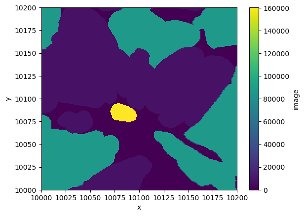
    *empty*

datatree.DataTree

• Groups: (5)
  <xarray.DatasetView>
  Dimensions:  (y: 17098, x: 70)
  Coordinates:
    * y        (y) float64 0.5 1.5 2.5 3.5 ... 1.71e+04 1.71e+04 1.71e+04
    * x        (x) float64 30.5 31.5 32.5 33.5 34.5 ... 95.5 96.5 97.5 98.5 99.5
  Data variables:
      image    (y, x) uint32 dask.array<chunksize=(4096, 70), meta=np.ndarray>

  scale0

  • Groups: (0)
  • Dimensions:
    • y: 17098
    • x: 70
  • Coordinates: (2)
    • y
      (y)
      float64
      0.5 1.5 2.5 ... 1.71e+04 1.71e+04

      array([5.00000e-01, 1.50000e+00, 2.50000e+00, ..., 1.70955e+04, 1.70965e+04,
             1.70975e+04])

    • x
      (x)
      float64
      30.5 31.5 32.5 ... 97.5 98.5 99.5

      array([30.5, 31.5, 32.5, 33.5, 34.5, 35.5, 36.5, 37.5, 38.5, 39.5, 40.5, 41.5,
             42.5, 43.5, 44.5, 45.5, 46.5, 47.5, 48.5, 49.5, 50.5, 51.5, 52.5, 53.5,
             54.5, 55.5, 56.5, 57.5, 58.5, 59.5, 60.5, 61.5, 62.5, 63.5, 64.5, 65.5,
             66.5, 67.5, 68.5, 69.5, 70.5, 71.5, 72.5, 73.5, 74.5, 75.5, 76.5, 77.5,
             78.5, 79.5, 80.5, 81.5, 82.5, 83.5, 84.5, 85.5, 86.5, 87.5, 88.5, 89.5,
             90.5, 91.5, 92.5, 93.5, 94.5, 95.5, 96.5, 97.5, 98.5, 99.5])

  • Data variables: (1)
    • image
      (y, x)
      uint32
      dask.array<chunksize=(4096, 70), meta=np.ndarray>

      transform :

      {'global': Identity }

      Array Chunk Bytes 4.57 MiB 1.09 MiB Shape (17098, 70) (4096, 70) Dask graph 5 chunks in 3 graph layers Data type uint32 numpy.ndarray

  • Attributes: (0)

  <xarray.DatasetView>
  Dimensions:  (y: 8549, x: 35)
  Coordinates:
    * y        (y) float64 1.0 3.0 5.0 7.0 ... 1.709e+04 1.71e+04 1.71e+04
    * x        (x) float64 31.0 33.0 35.0 37.0 39.0 ... 91.0 93.0 95.0 97.0 99.0
  Data variables:
      image    (y, x) uint32 dask.array<chunksize=(4096, 35), meta=np.ndarray>

  scale1

  • Groups: (0)
  • Dimensions:
    • y: 8549
    • x: 35
  • Coordinates: (2)
    • y
      (y)
      float64
      1.0 3.0 5.0 ... 1.71e+04 1.71e+04

      array([1.0000e+00, 3.0000e+00, 5.0000e+00, ..., 1.7093e+04, 1.7095e+04,
             1.7097e+04])

    • x
      (x)
      float64
      31.0 33.0 35.0 ... 95.0 97.0 99.0

      array([31.000606, 33.000645, 35.000684, 37.000723, 39.000762, 41.000801,
             43.00084 , 45.000879, 47.000918, 49.000957, 51.000996, 53.001035,
             55.001075, 57.001114, 59.001153, 61.001192, 63.001231, 65.00127 ,
             67.001309, 69.001348, 71.001387, 73.001426, 75.001465, 77.001504,
             79.001543, 81.001582, 83.001622, 85.001661, 87.0017  , 89.001739,
             91.001778, 93.001817, 95.001856, 97.001895, 99.001934])

  • Data variables: (1)
    • image
      (y, x)
      uint32
      dask.array<chunksize=(4096, 35), meta=np.ndarray>

      transform :

      {'global': Sequence Scale (y, x) [2. 2.00003907] Identity }

      Array Chunk Bytes 1.14 MiB 560.00 kiB Shape (8549, 35) (4096, 35) Dask graph 3 chunks in 3 graph layers Data type uint32 numpy.ndarray

  • Attributes: (0)

  <xarray.DatasetView>
  Dimensions:  (y: 4274, x: 18)
  Coordinates:
    * y        (y) float64 2.0 6.001 10.0 14.0 ... 1.709e+04 1.709e+04 1.71e+04
    * x        (x) float64 30.0 34.0 38.0 42.0 46.0 ... 86.01 90.01 94.01 98.01
  Data variables:
      image    (y, x) uint32 dask.array<chunksize=(4096, 18), meta=np.ndarray>

  scale2

  • Groups: (0)
  • Dimensions:
    • y: 4274
    • x: 18
  • Coordinates: (2)
    • y
      (y)
      float64
      2.0 6.001 ... 1.709e+04 1.71e+04

      array([2.000234e+00, 6.000702e+00, 1.000117e+01, ..., 1.708800e+04,
             1.709200e+04, 1.709600e+04])

    • x
      (x)
      float64
      30.0 34.0 38.0 ... 94.01 98.01

      array([30.001758, 34.001993, 38.002227, 42.002462, 46.002696, 50.002931,
             54.003165, 58.003399, 62.003634, 66.003868, 70.004103, 74.004337,
             78.004572, 82.004806, 86.005041, 90.005275, 94.00551 , 98.005744])

  • Data variables: (1)
    • image
      (y, x)
      uint32
      dask.array<chunksize=(4096, 18), meta=np.ndarray>

      transform :

      {'global': Sequence Scale (y, x) [4.00046795 4.00023445] Identity }

      Array Chunk Bytes 300.52 kiB 288.00 kiB Shape (4274, 18) (4096, 18) Dask graph 2 chunks in 3 graph layers Data type uint32 numpy.ndarray

  • Attributes: (0)

  <xarray.DatasetView>
  Dimensions:  (y: 2137, x: 8)
  Coordinates:
    * y        (y) float64 4.0 12.0 20.0 28.0 ... 1.708e+04 1.709e+04 1.709e+04
    * x        (x) float64 36.0 44.0 52.0 60.0 68.0 76.0 84.0 92.01
  Data variables:
      image    (y, x) uint32 dask.array<chunksize=(2137, 8), meta=np.ndarray>

  scale3

  • Groups: (0)
  • Dimensions:
    • y: 2137
    • x: 8
  • Coordinates: (2)
    • y
      (y)
      float64
      4.0 12.0 ... 1.709e+04 1.709e+04

      array([4.000468e+00, 1.200140e+01, 2.000234e+01, ..., 1.707800e+04,
             1.708600e+04, 1.709400e+04])

    • x
      (x)
      float64
      36.0 44.0 52.0 ... 76.0 84.0 92.01

      array([36.00211 , 44.002579, 52.003048, 60.003517, 68.003986, 76.004455,
             84.004923, 92.005392])

  • Data variables: (1)
    • image
      (y, x)
      uint32
      dask.array<chunksize=(2137, 8), meta=np.ndarray>

      transform :

      {'global': Sequence Scale (y, x) [8.00093589 8.0004689 ] Identity }

      Array Chunk Bytes 66.78 kiB 66.78 kiB Shape (2137, 8) (2137, 8) Dask graph 1 chunks in 3 graph layers Data type uint32 numpy.ndarray

  • Attributes: (0)

  <xarray.DatasetView>
  Dimensions:  (y: 1068, x: 4)
  Coordinates:
    * y        (y) float64 8.005 24.01 40.02 ... 1.706e+04 1.707e+04 1.709e+04
    * x        (x) float64 40.0 56.0 72.0 88.01
  Data variables:
      image    (y, x) uint32 dask.array<chunksize=(1068, 4), meta=np.ndarray>

  scale4

  • Groups: (0)
  • Dimensions:
    • y: 1068
    • x: 4
  • Coordinates: (2)
    • y
      (y)
      float64
      8.005 24.01 ... 1.707e+04 1.709e+04

      array([8.004682e+00, 2.401404e+01, 4.002341e+01, ..., 1.705798e+04,
             1.707399e+04, 1.709000e+04])

    • x
      (x)
      float64
      40.0 56.0 72.0 88.01

      array([40.002344, 56.003282, 72.00422 , 88.005158])

  • Data variables: (1)
    • image
      (y, x)
      uint32
      dask.array<chunksize=(1068, 4), meta=np.ndarray>

      transform :

      {'global': Sequence Scale (y, x) [16.0093633 16.00093779] Identity }

      Array Chunk Bytes 16.69 kiB 16.69 kiB Shape (1068, 4) (1068, 4) Dask graph 1 chunks in 3 graph layers Data type uint32 numpy.ndarray

  • Attributes: (0)

• Dimensions:
• Coordinates: (0)
• Data variables: (0)
• Attributes: (0)

Finally, let’s make a plot of a portion of a portion of the labels.

multiscale_labels["scale0"]["image"].sel(
    x=slice(10000, 10200), y=slice(10000, 10200)
).plot.imshow()

<matplotlib.image.AxesImage at 0x307db2f90>

Shapes (geopandas.GeoDataFrame)

A GeoDataFrame is an object that inherits from a pandas.DataFrame, and as such it supports the APIs that pandas provides, but also new powerful APIs for geometric manipulation.

gdf = sdata_xenium["cell_boundaries"]
gdf

	geometry
aaaadpbp-1	POLYGON ((205.062 1489.838, 204.213 1490.475, ...
aaaaficg-1	POLYGON ((200.812 1811.988, 199.538 1812.625, ...
aaabbaka-1	POLYGON ((177.013 2158.575, 175.525 2159.425, ...
aaabbjoo-1	POLYGON ((185.513 2156.238, 184.238 2157.3, 18...
aaablchg-1	POLYGON ((197.2 2191.938, 197.413 2192.15, 197...
...	...
ojaaphhh-1	POLYGON ((4551.538 1640.925, 4551.325 1641.138...
ojabeldf-1	POLYGON ((4437.212 1627.75, 4437 1627.963, 443...
ojacfbid-1	POLYGON ((4462.712 1575.05, 4462.288 1575.475,...
ojacfhhg-1	POLYGON ((4619.962 1452.863, 4619.75 1453.075,...
ojacpeii-1	POLYGON ((4620.175 1526.388, 4619.75 1526.812,...

162254 rows × 1 columns

The geometry column is what contains the spatial information.

gdf.geometry.iloc[3]

In spatialdata, we support only dataframes where all the geometries are polygons/multipolygons, either where all the geometries are shapely.Point and a column called radius is present.

One can add new regular columns to the dataframe.

gdf["cell_area"] = gdf.area
gdf

	geometry	cell_area
aaaadpbp-1	POLYGON ((205.062 1489.838, 204.213 1490.475, ...	65.273241
aaaaficg-1	POLYGON ((200.812 1811.988, 199.538 1812.625, ...	47.436672
aaabbaka-1	POLYGON ((177.013 2158.575, 175.525 2159.425, ...	115.961463
aaabbjoo-1	POLYGON ((185.513 2156.238, 184.238 2157.3, 18...	90.922142
aaablchg-1	POLYGON ((197.2 2191.938, 197.413 2192.15, 197...	116.932837
...	...	...
ojaaphhh-1	POLYGON ((4551.538 1640.925, 4551.325 1641.138...	25.084211
ojabeldf-1	POLYGON ((4437.212 1627.75, 4437 1627.963, 443...	4.628853
ojacfbid-1	POLYGON ((4462.712 1575.05, 4462.288 1575.475,...	5.621909
ojacfhhg-1	POLYGON ((4619.962 1452.863, 4619.75 1453.075,...	6.141260
ojacpeii-1	POLYGON ((4620.175 1526.388, 4619.75 1526.812,...	5.757876

162254 rows × 2 columns

Points(dask.DataFrame)

The dask.DataFrame class is a subclass of pandas.DataFrame that allows for lazy loading and lazy, distributed computation using Dask. This is used because generally points collections of spatial transcriptomics datasets are too big to be handled with regular pandas.DataFrame objects.

When you perform operations on a dask.DataFrame, they are not computed until you choose to do so.

ddf = sdata_xenium["transcripts"]
ddf

Dask DataFrame Structure:

	x	y	z	feature_name	cell_id	transcript_id	fov_name	codeword_index	overlaps_nucleus	nucleus_distance	qv
npartitions=4
	float32	float32	float32	category[unknown]	string	uint64	string	int32	uint8	float32	float32
	...	...	...	...	...	...	...	...	...	...	...
	...	...	...	...	...	...	...	...	...	...	...
	...	...	...	...	...	...	...	...	...	...	...
	...	...	...	...	...	...	...	...	...	...	...

Dask Name: read-parquet, 1 graph layer

subset = ddf[ddf.feature_name == "CXCR4"][["feature_name", "cell_id"]]
subset

Dask DataFrame Structure:

	feature_name	cell_id
npartitions=4
	category[unknown]	string
	...	...
	...	...
	...	...
	...	...

Dask Name: getitem, 5 graph layers

Let’s now perform the operations by calling .compute().

df = subset.compute()
df

	feature_name	cell_id
2	CXCR4	UNASSIGNED
3	CXCR4	UNASSIGNED
213	CXCR4	UNASSIGNED
214	CXCR4	UNASSIGNED
272	CXCR4	UNASSIGNED
...	...	...
163229	CXCR4	UNASSIGNED
163244	CXCR4	jgdldkap-1
163270	CXCR4	jgebeofm-1
163279	CXCR4	jgcgjopd-1
164996	CXCR4	UNASSIGNED

78139 rows × 2 columns

As you can see, df is a regular pandas.DataFrame:

type(df)

pandas.core.frame.DataFrame

Tables(anndata.AnnData)

Finally we use AnnData objects to store annotations. We introduced the jargon tables to denotes these objects; please keep in mind that AnnData objects allow for storing dataframes and sparse/dense tensors.

adata = sdata_xenium["table"]
adata

AnnData object with n_obs × n_vars = 162254 × 377
    obs: 'cell_id', 'transcript_counts', 'control_probe_counts', 'control_codeword_counts', 'unassigned_codeword_counts', 'deprecated_codeword_counts', 'total_counts', 'cell_area', 'nucleus_area', 'region', 'z_level', 'nucleus_count', 'cell_labels'
    var: 'gene_ids', 'feature_types', 'genome'
    uns: 'spatialdata_attrs'
    obsm: 'spatial'

Let’s see some examples. A gene expression matrix can be stored the .X slot.

adata.X

<Compressed Sparse Row sparse matrix of dtype 'float32'
	with 4900367 stored elements and shape (162254, 377)>

adata.to_df()

	ABCC11	ACE2	ACKR1	ACTA2	ACTG2	ADAM28	ADAMTS1	ADGRE1	ADGRL4	ADH1C	...	TRAC	TREM2	TSPAN19	UBE2C	UMOD	UPK3B	VCAN	VSIG4	VWA5A	VWF
0	0.0	0.0	0.0	0.0	0.0	0.0	0.0	0.0	0.0	0.0	...	0.0	0.0	0.0	0.0	0.0	0.0	0.0	0.0	0.0	0.0
1	0.0	0.0	0.0	0.0	1.0	0.0	0.0	0.0	0.0	0.0	...	2.0	0.0	0.0	0.0	0.0	0.0	0.0	0.0	0.0	0.0
2	0.0	0.0	0.0	0.0	1.0	1.0	0.0	0.0	0.0	0.0	...	0.0	0.0	0.0	0.0	0.0	0.0	0.0	0.0	0.0	0.0
3	0.0	0.0	0.0	0.0	0.0	1.0	0.0	0.0	0.0	0.0	...	0.0	0.0	0.0	0.0	0.0	0.0	0.0	0.0	0.0	0.0
4	0.0	0.0	0.0	0.0	0.0	0.0	0.0	0.0	0.0	0.0	...	0.0	0.0	0.0	0.0	0.0	0.0	0.0	1.0	0.0	1.0
...	...	...	...	...	...	...	...	...	...	...	...	...	...	...	...	...	...	...	...	...	...
162249	0.0	0.0	0.0	0.0	0.0	0.0	0.0	0.0	0.0	0.0	...	0.0	0.0	0.0	0.0	0.0	0.0	0.0	0.0	0.0	0.0
162250	0.0	0.0	0.0	0.0	0.0	0.0	0.0	0.0	0.0	0.0	...	0.0	0.0	0.0	0.0	0.0	0.0	0.0	0.0	0.0	0.0
162251	0.0	0.0	0.0	0.0	0.0	0.0	0.0	0.0	0.0	0.0	...	0.0	0.0	0.0	0.0	0.0	0.0	0.0	0.0	0.0	0.0
162252	0.0	0.0	0.0	0.0	0.0	0.0	0.0	0.0	0.0	0.0	...	0.0	0.0	0.0	0.0	0.0	0.0	0.0	0.0	0.0	0.0
162253	0.0	0.0	0.0	0.0	0.0	0.0	0.0	0.0	0.0	0.0	...	0.0	0.0	0.0	0.0	0.0	0.0	0.0	0.0	0.0	0.0

162254 rows × 377 columns

Information on the genes (=variables), is stored in the .var slot.

adata.var

	gene_ids	feature_types	genome
ABCC11	ENSG00000121270	Gene Expression	Unknown
ACE2	ENSG00000130234	Gene Expression	Unknown
ACKR1	ENSG00000213088	Gene Expression	Unknown
ACTA2	ENSG00000107796	Gene Expression	Unknown
ACTG2	ENSG00000163017	Gene Expression	Unknown
...	...	...	...
UPK3B	ENSG00000243566	Gene Expression	Unknown
VCAN	ENSG00000038427	Gene Expression	Unknown
VSIG4	ENSG00000155659	Gene Expression	Unknown
VWA5A	ENSG00000110002	Gene Expression	Unknown
VWF	ENSG00000110799	Gene Expression	Unknown

377 rows × 3 columns

Information on the cells (=observations), is stored in the .obs slot.

adata.obs

	cell_id	transcript_counts	control_probe_counts	control_codeword_counts	unassigned_codeword_counts	deprecated_codeword_counts	total_counts	cell_area	nucleus_area	region	z_level	nucleus_count	cell_labels
0	aaaadpbp-1	0	0	0	0	0	0	68.456877	NaN	cell_circles	0.0	0.0	1
1	aaaaficg-1	19	0	0	0	0	19	49.130002	21.268595	cell_circles	0.0	1.0	2
2	aaabbaka-1	53	0	0	0	0	53	119.618911	74.778753	cell_circles	0.0	1.0	3
3	aaabbjoo-1	29	0	0	0	0	29	94.241097	59.109533	cell_circles	0.0	1.0	4
4	aaablchg-1	42	0	0	1	0	43	120.341411	52.426408	cell_circles	0.0	1.0	5
...	...	...	...	...	...	...	...	...	...	...	...	...	...
162249	ojaaphhh-1	3	0	0	0	0	3	26.913126	11.153594	cell_circles	5.0	1.0	162250
162250	ojabeldf-1	6	0	0	0	0	6	5.418750	5.418750	cell_circles	7.0	1.0	162251
162251	ojacfbid-1	0	0	0	0	0	0	6.502500	6.502500	cell_circles	5.0	1.0	162252
162252	ojacfhhg-1	2	0	0	0	0	2	7.089532	7.089532	cell_circles	5.0	1.0	162253
162253	ojacpeii-1	1	0	0	0	0	1	6.683125	6.683125	cell_circles	5.0	1.0	162254

162254 rows × 13 columns

The slot .uns can contain unstructured data. In particular it contains some metadata that is used to link tables to the spatial elements (e.g. cell segmentation masks) that they annotate.

adata.uns

{'spatialdata_attrs': {'instance_key': 'cell_id',
  'region': 'cell_circles',
  'region_key': 'region'}}

image = sdata_visium.images[
    "CytAssist_FFPE_Protein_Expression_Human_Glioblastoma_hires_image"
]
print(image.data)
image.data

dask.array<from-zarr, shape=(3, 2000, 1744), dtype=uint8, chunksize=(3, 2000, 1744), chunktype=numpy.ndarray>

Array Chunk Bytes 9.98 MiB 9.98 MiB Shape (3, 2000, 1744) (3, 2000, 1744) Dask graph 1 chunks in 2 graph layers Data type uint8 numpy.ndarray

As you can see, xarray is using dask internally. You can compute the data as follows:

# produces an xarray object that is fully-loaded in memory
image.compute()

<xarray.DataArray 'image' (c: 1, y: 522, x: 575)>
array([[[0, 0, 0, ..., 0, 0, 0],
        [0, 0, 0, ..., 0, 0, 0],
        [0, 0, 0, ..., 0, 0, 0],
        ...,
        [0, 0, 0, ..., 0, 0, 0],
        [0, 0, 0, ..., 0, 0, 0],
        [0, 0, 0, ..., 0, 0, 0]]], dtype=uint8)
Coordinates:
  * c        (c) int64 0
  * y        (y) float64 0.5 1.5 2.5 3.5 4.5 ... 517.5 518.5 519.5 520.5 521.5
  * x        (x) float64 0.5 1.5 2.5 3.5 4.5 ... 570.5 571.5 572.5 573.5 574.5
Attributes:
    transform:  {'global': Sequence \n    Scale (c, y, x)\n        [1.       ...

xarray.DataArray

'image'

• c: 1
• y: 522
• x: 575

• 0 0 0 0 0 0 0 0 0 0 0 0 0 0 0 0 0 ... 0 0 0 0 0 0 0 0 0 0 0 0 0 0 0 0

  array([[[0, 0, 0, ..., 0, 0, 0],
          [0, 0, 0, ..., 0, 0, 0],
          [0, 0, 0, ..., 0, 0, 0],
          ...,
          [0, 0, 0, ..., 0, 0, 0],
          [0, 0, 0, ..., 0, 0, 0],
          [0, 0, 0, ..., 0, 0, 0]]], dtype=uint8)

• Coordinates: (3)
  • c
    (c)
    int64
    0

    array([0])

  • y
    (y)
    float64
    0.5 1.5 2.5 ... 519.5 520.5 521.5

    array([5.000e-01, 1.500e+00, 2.500e+00, ..., 5.195e+02, 5.205e+02, 5.215e+02])

  • x
    (x)
    float64
    0.5 1.5 2.5 ... 572.5 573.5 574.5

    array([5.000e-01, 1.500e+00, 2.500e+00, ..., 5.725e+02, 5.735e+02, 5.745e+02])

• Indexes: (3)
  • c
    PandasIndex

    PandasIndex(Index([0], dtype='int64', name='c'))

  • y
    PandasIndex

    PandasIndex(Index([  0.5,   1.5,   2.5,   3.5,   4.5,   5.5,   6.5,   7.5,   8.5,   9.5,
           ...
           512.5, 513.5, 514.5, 515.5, 516.5, 517.5, 518.5, 519.5, 520.5, 521.5],
          dtype='float64', name='y', length=522))

  • x
    PandasIndex

    PandasIndex(Index([  0.5,   1.5,   2.5,   3.5,   4.5,   5.5,   6.5,   7.5,   8.5,   9.5,
           ...
           565.5, 566.5, 567.5, 568.5, 569.5, 570.5, 571.5, 572.5, 573.5, 574.5],
          dtype='float64', name='x', length=575))

• Attributes: (1)

  transform :

  {'global': Sequence Scale (c, y, x) [1. 3.86311352 3.50777513] Translation (c, y, x) [ 0. 4548. 1154.]}

# accesses the data inside xarray, as a numpy array object
x = image.compute().data
print(type(x))
x

<class 'numpy.ndarray'>

array([[[0, 0, 0, ..., 0, 0, 0],
        [0, 0, 0, ..., 0, 0, 0],
        [0, 0, 0, ..., 0, 0, 0],
        ...,
        [0, 0, 0, ..., 0, 0, 0],
        [0, 0, 0, ..., 0, 0, 0],
        [0, 0, 0, ..., 0, 0, 0]]], dtype=uint8)

Futher reading

As mentioned before, we invite the readers to become familiar with the geospatial Python data structures that we use in the spatialdata library. In the next tutorials we will explore various functions enabled by the spatialdata framework; anyway for a deeper introduction we kindly point you to the notebooks section of the documentation, and in particular to the following notebooks, which explain in detail how to create SpatialData objects from screatch and manipulate them:

• In depth introduction to SpatialData objects.

• In depth introduction to spatial elements and models (.parse(), .validate()).

• Annotating elements and manipulating annotations.

Furthermore, you can find curated code examples by checking the various readers available in the spatialdata-io library.

Finally, for a deeper description of all the available functions, please consult the API documentation.