Colouring by expression: tables, layers, and gene symbols

When you colour an element by a gene, spatialdata-plot reads the value from the table that annotates it. Three arguments control exactly which values it uses: table_name (which table), table_layer (which matrix within that table), and gene_symbols (how to look a gene up in var). By the end you should be able to:

• Colour spots by a gene’s expression.

• Read from a specific matrix with table_layer (e.g. raw counts vs a normalised layer).

• Look genes up by symbol when var is indexed by IDs, with gene_symbols.

• Choose between several annotating tables with table_name.

We use the real 10x Visium mouse-brain dataset from squidpy. It ships with a single raw table, so we construct the extra layer, the gene-ID index, and the second table in-notebook to demonstrate each argument — real datasets often already carry them.

Setup

import numpy as np
import scipy.sparse as sp
import anndata as ad
import squidpy as sq
from spatialdata import SpatialData
from spatialdata.models import TableModel

import spatialdata_plot  # noqa: F401  # registers the .pl accessor

sdata = sq.datasets.visium_hne_sdata()
table = sdata.tables["adata"]
gene = "Mbp"  # myelin basic protein, a white-matter marker
sdata

INFO     Loading existing dataset from data/spatialdata/visium_hne_sdata.zarr

SpatialData object, with associated Zarr store: /Users/tim.treis/Documents/GitHub/spatialdata-plot/docs/notebooks/examples/data/spatialdata/visium_hne_sdata.zarr
├── Images
│     └── 'hne': DataTree[cyx] (3, 11757, 11291), (3, 5878, 5645), (3, 2939, 2822), (3, 1469, 1411)
├── Shapes
│     └── 'spots': GeoDataFrame shape: (2688, 2) (2D shapes)
└── Tables
      └── 'adata': AnnData (2688, 18078)
with coordinate systems:
    ▸ 'global', with elements:
        hne (Images), spots (Shapes)

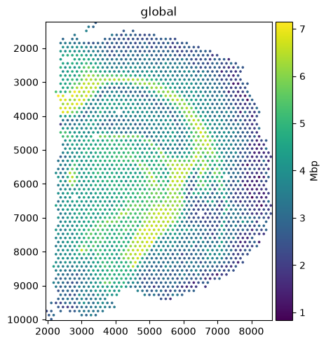
1. Colour by a gene

Passing a var name to color= colours each spot by that gene’s expression, from the annotating table’s main matrix (X).

sdata.pl.render_shapes("spots", color=gene).pl.show()

2. Choosing the matrix — table_layer

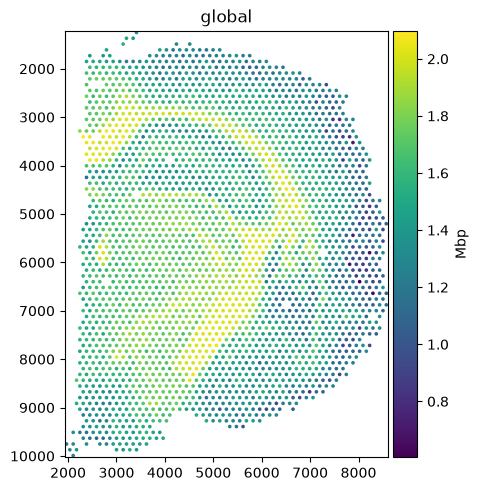
A table can hold several matrices in .layers (raw counts, normalised, scaled). table_layer= picks which one to colour from. Here we add a log-normalised layer and compare it with the raw X above — the log scale compresses the bright outliers and reveals more structure.

(Setup — real data often already carries such a layer.) Note table_layer only affects gene-expression colouring, i.e. a var_names lookup; colouring by an obs column ignores it.

# setup: add a normalised layer (your data may already have one)
raw = table.X.toarray() if sp.issparse(table.X) else table.X
table.layers["lognorm"] = np.log1p(raw)

sdata.pl.render_shapes("spots", color=gene, table_layer="lognorm").pl.show()

3. Looking up by symbol — gene_symbols

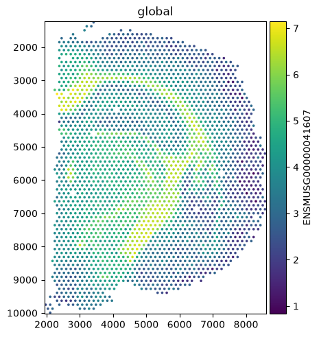
Many datasets index var by a stable ID (Ensembl) and keep the human-readable symbol in a column. color= then can’t find a symbol directly. gene_symbols= names the column to map through. We simulate that layout on a copy of the table and render it through a throwaway SpatialData, so the original table stays symbol-indexed and every earlier cell keeps working.

# setup — skip on your own data: simulate an ID-indexed table on a copy so the original is untouched
table_ids = table.copy()
table_ids.var["symbol"] = table_ids.var_names
table_ids.var.index = list(table_ids.var["gene_ids"].values)  # var now indexed by Ensembl IDs

# render from a lightweight SpatialData that reuses the spots and the copied, ID-indexed table
# color= still takes the symbol; gene_symbols tells the renderer which var column to map through
demo = SpatialData(shapes={"spots": sdata.shapes["spots"]}, tables={"adata": table_ids})
demo.pl.render_shapes("spots", color=gene, gene_symbols="symbol").pl.show()

4. Choosing the table — table_name

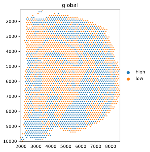
An element can be annotated by more than one table. When there is only one, it is used automatically; with several you disambiguate with table_name=. We add a second table of per-spot QC flags and colour by it.

A table links to its element through three keys in table.uns['spatialdata_attrs']: region (the annotated element), region_key (the obs column naming that element for each row), and instance_key (the obs column giving each row’s id within it). We assemble the two tables into a throwaway SpatialData so the original object is left untouched.

attrs = table.uns["spatialdata_attrs"]
region_key = attrs["region_key"]      # obs column naming which element each row annotates
instance_key = attrs["instance_key"]  # obs column giving the row id within that element
region = attrs["region"]              # the annotated element ("spots")

qc_obs = table.obs[[region_key, instance_key]].copy()
qc_obs["qc"] = np.where(table.obs["total_counts"] > table.obs["total_counts"].median(), "high", "low")
qc_table = TableModel.parse(
    ad.AnnData(obs=qc_obs), region=region, region_key=region_key, instance_key=instance_key
)

# two tables annotate the same spots; table_name picks which one to colour from
demo = SpatialData(shapes={"spots": sdata.shapes["spots"]}, tables={"adata": table, "qc": qc_table})
demo.pl.render_shapes("spots", color="qc", table_name="qc").pl.show()

WARNING  render_shapes: Converting copy of 'qc' column to categorical dtype for categorical plotting. Consider     
         converting before plotting.

Summary

• Colouring by a gene reads from the annotating table of the element.

• table_layer= selects the matrix within that table (e.g. raw X vs a lognorm layer), for gene-expression colouring only — an obs-column colour ignores it.

• gene_symbols= names the var column of symbols to look color= up in, for ID-indexed tables.

• table_name= picks the table when an element has more than one; with a single table it is automatic.

Together these let you point render_* at exactly the values you want to visualise, without reshaping your SpatialData object.

For reproducibility

# ruff: noqa: F401, F811, I001, E402
# fmt: off
import warnings
import spatialdata_plot

%load_ext watermark
# fmt: on

%watermark -v -m -p spatialdata,spatialdata_plot,squidpy,anndata,numpy

Python implementation: CPython
Python version       : 3.14.6
IPython version      : 9.14.1

spatialdata     : 0.7.3
spatialdata_plot: 0.4.1
squidpy         : 1.8.2
anndata         : 0.12.17
numpy           : 2.4.6

Compiler    : Clang 20.1.8 
OS          : Darwin
Release     : 25.2.0
Machine     : arm64
Processor   : arm
CPU cores   : 8
Architecture: 64bit