Legends and colorbars in spatialdata-plot

Every coloured plot needs a key. spatialdata-plot builds three kinds automatically: a categorical colour (named groups) gets a legend, a continuous colour (a numeric range) gets a colorbar, and a multichannel image gets a channel legend. show() places and styles the legend and colorbar; the channel legend is switched on with render_images(channels_as_legend=True). By the end you should be able to:

• Place a categorical legend anywhere (legend_loc) and restyle it (legend_fontsize, legend_fontweight, legend_fontoutline, legend_title), or bundle those in legend_params.

• Control which categories appear with na_in_legend.

• Place and style a colorbar with colorbar / colorbar_params.

• Label a multichannel composite with channels_as_legend.

• Combine keys across a multi-panel figure.

We use the real 10x Visium mouse-brain dataset from squidpy for the legend and colorbar, and the Xenium cells fluorescence image for the channel legend — both cached on first use.

Setup

import squidpy as sq

import spatialdata_plot  # noqa: F401  # registers the .pl accessor

sdata = sq.datasets.visium_hne_sdata()
sdata

INFO     Loading existing dataset from data/spatialdata/visium_hne_sdata.zarr

SpatialData object, with associated Zarr store: /Users/tim.treis/Documents/GitHub/spatialdata-plot/docs/notebooks/examples/data/spatialdata/visium_hne_sdata.zarr
├── Images
│     └── 'hne': DataTree[cyx] (3, 11757, 11291), (3, 5878, 5645), (3, 2939, 2822), (3, 1469, 1411)
├── Shapes
│     └── 'spots': GeoDataFrame shape: (2688, 2) (2D shapes)
└── Tables
      └── 'adata': AnnData (2688, 18078)
with coordinate systems:
    ▸ 'global', with elements:
        hne (Images), spots (Shapes)

1. The default categorical legend

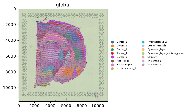
Colouring by a categorical column draws a legend automatically. cluster holds named brain regions; we render the spots over the H&E image.

(
    sdata.pl.render_images("hne")
    .pl.render_shapes("spots", color="cluster")
).pl.show(legend_fontsize=6)

2. Placing the legend — legend_loc

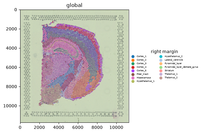
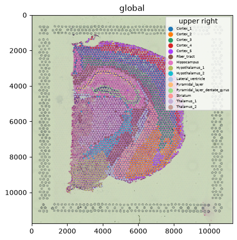
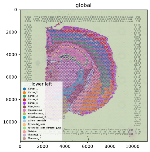
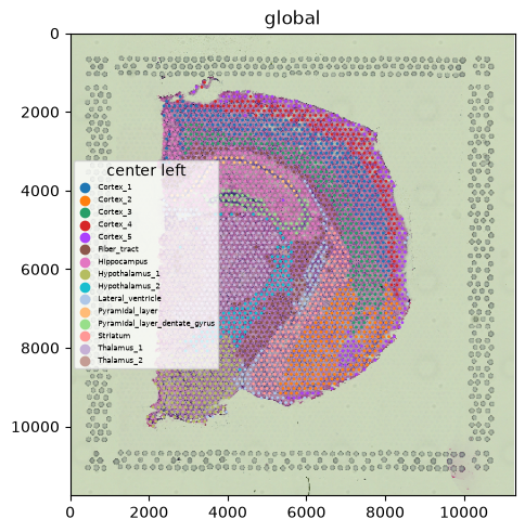
legend_loc takes any matplotlib location ("upper right", "lower left", "center left", …) or "right margin" to park the legend outside the axes. The margin keeps the legend off the data; the matplotlib locations place it on top. Here are four placements of the same plot.

for loc in ["right margin", "upper right", "lower left", "center left"]:
    (
        sdata.pl.render_images("hne")
        .pl.render_shapes("spots", color="cluster")
    ).pl.show(legend_loc=loc, legend_fontsize=5, legend_title=loc)

3. Restyling the legend

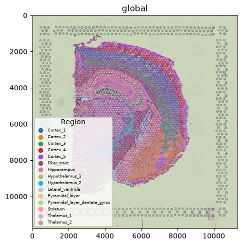
legend_fontsize, legend_fontweight, and legend_fontoutline (a contrasting outline around the text, useful over busy images) style the entries; legend_title names it.

(
    sdata.pl.render_images("hne")
    .pl.render_shapes("spots", color="cluster")
).pl.show(
    legend_loc="lower left",
    legend_fontsize=6,
    legend_fontweight="bold",
    legend_fontoutline=2,
    legend_title="Region",
)

4. Hiding NA — na_in_legend

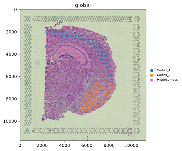
groups subsets a categorical colour to the named categories; the remaining spots become NA, and na_in_legend=False drops that NA entry from the key.

(
    sdata.pl.render_images("hne")
    .pl.render_shapes("spots", color="cluster", groups=["Cortex_1", "Cortex_2", "Hippocampus"])
).pl.show(na_in_legend=False, legend_fontsize=7)

5. Bundling options — legend_params

Instead of the flat legend_* kwargs you can pass one legend_params dict. Accepted keys: location (or loc), fontsize, fontweight, fontoutline, na_in_legend; it overrides the matching flat kwargs, and unknown keys raise an error.

Note legend_title is not among the accepted keys — keep it as a flat legend_title= kwarg.

(
    sdata.pl.render_images("hne")
    .pl.render_shapes("spots", color="cluster")
).pl.show(
    legend_params={"loc": "right margin", "fontsize": 6, "fontweight": "bold"},
)

6. Continuous colours get a colorbar

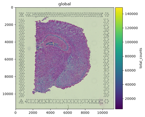
Colouring by a continuous column draws a colorbar instead of a legend. Here, total counts per spot. colorbar=True is the default; pass colorbar=False to suppress it.

(
    sdata.pl.render_images("hne")
    .pl.render_shapes("spots", color="total_counts")
).pl.show()

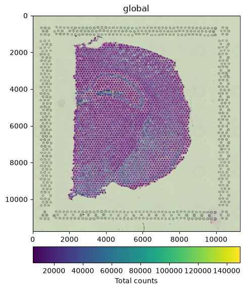
7. Placing and styling the colorbar — colorbar_params

colorbar_params accepts label, loc (position — "right" by default, or "left"/"top"/ "bottom"), width, pad, plus matplotlib colorbar keys. Set loc to move the bar; its orientation follows the side automatically (horizontal for top/bottom). Passing only orientation does not move it — the bar stays docked right.

(
    sdata.pl.render_images("hne")
    .pl.render_shapes("spots", color="total_counts")
).pl.show(
    colorbar_params={"loc": "bottom", "label": "Total counts"},
)

8. Labelling a multichannel image — channels_as_legend

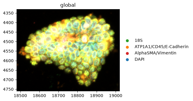
A multichannel image has no single colour to key, so channels_as_legend=True adds a channel legend mapping each channel to its rendered colour. We switch to the Xenium cells fluorescence image, whose channels are named markers (see the Multichannel & fluorescence images tutorial).

from spatialdata_plot import PercentileNormalize

cells = sq.datasets.cells()
n_channels = 4
cells.pl.render_images(
    "morphology_focus",
    norm=[PercentileNormalize(1, 99)] * n_channels,
    channels_as_legend=True,
).pl.show()

INFO     Loading existing dataset from data/spatialdata/cells.zarr

9. Several keys in one figure

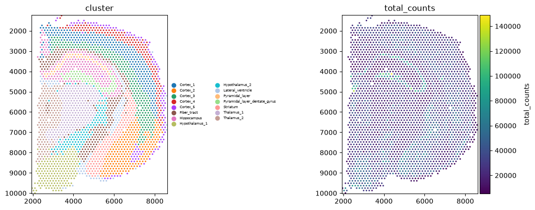
Passing a list to color= renders one panel per colouring (see the Multi-panel colouring tutorial). Each panel gets the right key: a legend for the categorical panel, a colorbar for the continuous one.

(
    sdata.pl.render_shapes("spots", color=["cluster", "total_counts"])
).pl.show(ncols=2, legend_fontsize=5)

Summary

• Categorical colours draw a legend, continuous colours a colorbar, and multichannel images a channel legend (channels_as_legend) — all automatically.

• Place the legend with legend_loc (matplotlib locations or "right margin"), and style it with legend_fontsize/fontweight/fontoutline, legend_title, na_in_legend; or bundle in legend_params.

• Place and style the colorbar with colorbar_params; loc ("right"/"left"/"top"/"bottom") sets its position and the orientation follows.

• In a multi-panel color=[...] figure each panel gets the appropriate key.

For reproducibility

# ruff: noqa: F401, F811, I001, E402
# fmt: off
import warnings
import spatialdata_plot

%load_ext watermark
# fmt: on

%watermark -v -m -p spatialdata,spatialdata_plot,squidpy,matplotlib,numpy

Python implementation: CPython
Python version       : 3.14.6
IPython version      : 9.14.1

spatialdata     : 0.7.3
spatialdata_plot: 0.4.1
squidpy         : 1.8.2
matplotlib      : 3.11.0
numpy           : 2.4.6

Compiler    : Clang 20.1.8 
OS          : Darwin
Release     : 25.2.0
Machine     : arm64
Processor   : arm
CPU cores   : 8
Architecture: 64bit