Colour and palettes in spatialdata-plot

This tutorial covers how spatialdata-plot decides what colours to draw, and the helpers it ships for building palettes. By the end you should be able to:

• Reason about where a colour comes from when you write color=....

• Use groups to focus on a subset of categories without throwing the rest away.

• Build perceptually well-spaced and colourblind-safe palettes with make_palette and make_palette_from_data.

We use the synthetic blobs dataset throughout so the notebook stays small and reproducible.

Setup

import numpy as np
import pandas as pd
import matplotlib.pyplot as plt

import spatialdata as sd
import spatialdata_plot as sdp  # registers the .pl accessor; also aliased for sdp.pl.make_palette below

sdata = sd.datasets.blobs()
sdata

SpatialData object
├── Images
│     ├── 'blobs_image': DataArray[cyx] (3, 512, 512)
│     └── 'blobs_multiscale_image': DataTree[cyx] (3, 512, 512), (3, 256, 256), (3, 128, 128)
├── Labels
│     ├── 'blobs_labels': DataArray[yx] (512, 512)
│     └── 'blobs_multiscale_labels': DataTree[yx] (512, 512), (256, 256), (128, 128)
├── Points
│     └── 'blobs_points': DataFrame with shape: (<Delayed>, 4) (2D points)
├── Shapes
│     ├── 'blobs_circles': GeoDataFrame shape: (5, 2) (2D shapes)
│     ├── 'blobs_multipolygons': GeoDataFrame shape: (2, 1) (2D shapes)
│     └── 'blobs_polygons': GeoDataFrame shape: (5, 1) (2D shapes)
└── Tables
      └── 'table': AnnData (26, 3)
with coordinate systems:
    ▸ 'global', with elements:
        blobs_image (Images), blobs_multiscale_image (Images), blobs_labels (Labels), blobs_multiscale_labels (Labels), blobs_points (Points), blobs_circles (Shapes), blobs_multipolygons (Shapes), blobs_polygons (Shapes)

We need a categorical column with a few levels to show off palettes. blobs ships with a 2-category genes column on the points, so we synthesise a 5-category cell_type annotation on the labels table and a region_type on blobs_polygons to exercise the column-on-element path.

rng = np.random.default_rng(0)

# Categorical on the table (annotates blobs_labels)
table = sdata.tables['table']
table.obs['cell_type'] = pd.Categorical(
    rng.choice(['A', 'B', 'C', 'D', 'E'], size=table.n_obs),
    categories=['A', 'B', 'C', 'D', 'E'],
)

# Categorical directly on a shapes GeoDataFrame
sdata.shapes['blobs_polygons']['region_type'] = pd.Categorical(
    ['stroma', 'tumour', 'stroma', 'immune', 'tumour'],
)

table.obs['cell_type'].value_counts().sort_index()

cell_type
A    5
B    4
C    4
D    6
E    7
Name: count, dtype: int64

1. Where does my colour come from?

When you pass color= to a render_* function, spatialdata-plot resolves it in a fixed order:

1. Literal colour — if the string parses as a colour (hex like '#ff0000', a named matplotlib colour, or an RGB(A) tuple), it’s used directly.

2. Column name — otherwise it’s looked up on the element itself (the GeoDataFrame for shapes/points), then on the linked AnnData table’s obs (or var for gene expression).

3. Stored colours — for a categorical column, if no palette= is given, the matching adata.uns['<column>_colors'] entry is honoured (the AnnData convention scanpy writes).

Because step 1 wins, a few matplotlib shorthands that commonly collide with gene or column names are deliberately rejected so they fall through to the column lookup: greyscale strings ('0', '0.5', '1'), single-letter colours ('r', 'g', 'b', …), the Cn cycle ('C0', 'C1', …), and tab:/xkcd: prefixes. A column named 'red', on the other hand, is still parseable as a colour and would be misread — rename it before plotting.

The next three cells walk through each branch.

Literal colour

sdata.pl.render_shapes('blobs_polygons', color='#1f77b4').pl.show()

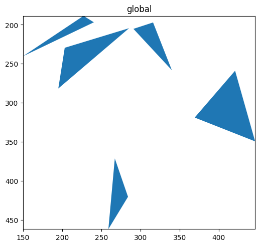
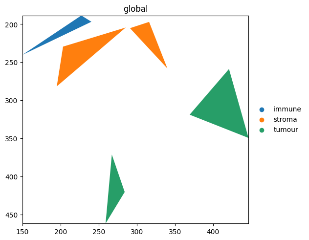
Column on the element

region_type lives directly on the blobs_polygons GeoDataFrame. It is found there first, so no table lookup is needed.

sdata.pl.render_shapes('blobs_polygons', color='region_type').pl.show()

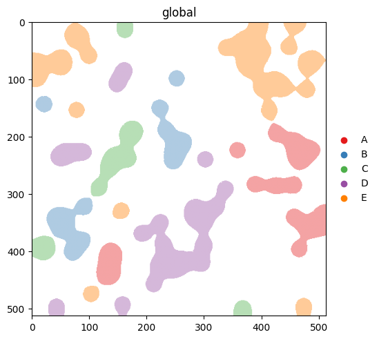
Stored colours in .uns

If you’ve already coloured a categorical column elsewhere (e.g. in scanpy), the matching '<column>_colors' entry in .uns is honoured automatically. Setting it explicitly:

table.uns['cell_type_colors'] = ['#e41a1c', '#377eb8', '#4daf4a', '#984ea3', '#ff7f00']
sdata.pl.render_labels('blobs_labels', color='cell_type').pl.show()
print('rendered with:', table.uns['cell_type_colors'])

rendered with: ['#e41a1c', '#377eb8', '#4daf4a', '#984ea3', '#ff7f00']

An explicit palette= argument overrides .uns. The precedence is: explicit palette= > .uns['<col>_colors'] > scanpy defaults. Compare this output with the next section, where we clear .uns['cell_type_colors'] and let the scanpy defaults take over.

2. Categorical vs continuous

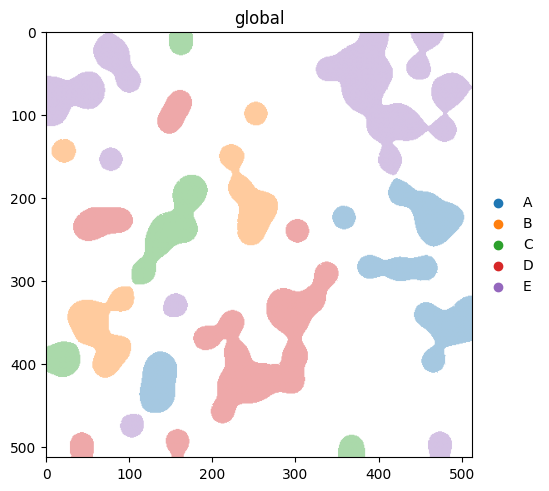
spatialdata-plot infers whether a column is categorical or continuous from its dtype. Categorical columns use palette=; continuous columns use cmap=. We clear the .uns['cell_type_colors'] we set above so this section actually exercises the scanpy fallback.

del table.uns['cell_type_colors']

(
    sdata.pl.render_labels('blobs_labels', color='cell_type')  # categorical -> palette
    .pl.show()
)

(
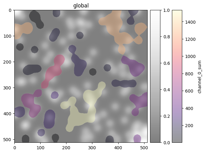
    sdata.pl.render_images('blobs_image', channel=0, cmap='Greys_r', alpha=0.5)
    .pl.render_labels('blobs_labels', color='channel_0_sum', cmap='magma')  # continuous -> cmap
    .pl.show()
)

3. Focusing on a subset with groups

groups= selects categories to highlight. As of v0.3.0, non-matching elements are hidden by default. If you’d rather see them in a neutral colour, pass na_color.

Default: non-group elements hidden

sdata.pl.render_labels('blobs_labels', color='cell_type', groups=['A', 'B']).pl.show()

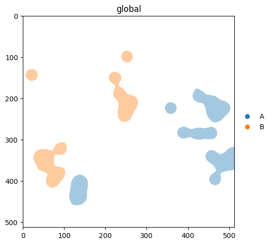
With na_color: non-group elements rendered in a neutral colour

(
    sdata.pl.render_labels(
        'blobs_labels',
        color='cell_type',
        groups=['A', 'B'],
        na_color='lightgrey',
    )
    .pl.show()
)

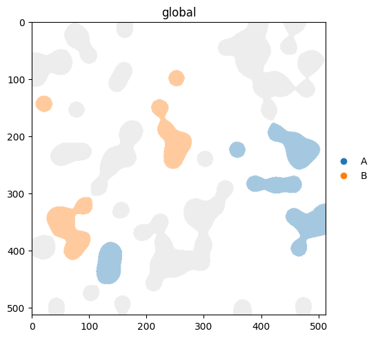
v0.3.0 note. Earlier versions rendered non-matching categories in the default NA colour by default. Now the default is to hide them, and you opt back into the old behaviour by passing na_color. Pass na_color='lightgrey' (or any colour) any time you want context, not just focus.

4. Building palettes with make_palette

make_palette(n, palette=..., method=...) returns a list of n hex colours. Two knobs:

• palette controls which colours are sampled. Accepts None (scanpy defaults), a list, a named palette like 'okabe_ito', or any matplotlib colormap name.

• method controls how they’re ordered. 'default' keeps source order; 'contrast' reorders for maximum pairwise perceptual distance; 'colorblind' reorders for the worst-case CVD type; 'protanopia' / 'deuteranopia' / 'tritanopia' reorder for a specific CVD type.

A small helper to inspect a palette as a strip of swatches:

def show_palette(colors: list[str], title: str = '') -> None:
    fig, ax = plt.subplots(figsize=(len(colors) * 0.6, 0.8))
    for i, c in enumerate(colors):
        ax.add_patch(plt.Rectangle((i, 0), 1, 1, color=c))
    ax.set_xlim(0, len(colors))
    ax.set_ylim(0, 1)
    ax.set_xticks([])
    ax.set_yticks([])
    ax.set_title(title, loc='left')
    plt.show()

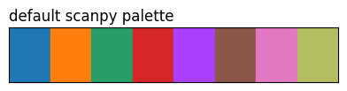
show_palette(sdp.pl.make_palette(8), 'default scanpy palette')
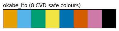
show_palette(sdp.pl.make_palette(8, palette='okabe_ito'), "okabe_ito (8 CVD-safe colours)")
show_palette(sdp.pl.make_palette(8, palette='tab10'), 'tab10, source order')
show_palette(sdp.pl.make_palette(8, palette='tab10', method='contrast'), "tab10, method='contrast'")
show_palette(sdp.pl.make_palette(8, palette='tab10', method='colorblind'), "tab10, method='colorblind'")
show_palette(sdp.pl.make_palette(8, palette='tab10', method='deuteranopia'), "tab10, method='deuteranopia'")

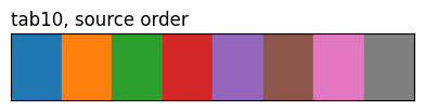
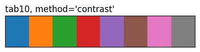
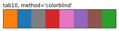
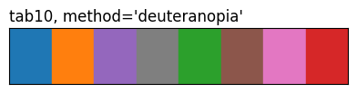
The three tab10 rows highlight what method does: same eight source colours, different ordering. 'contrast' and the CVD methods reorder by pairwise perceptual distance (under normal vision or a simulated deficiency), so the first few entries are spread further apart than they’d be in source order.

5. Palettes that already know your categories

make_palette_from_data(sdata, element, color, ...) returns a {category: hex} dictionary you can pass straight back into a render call. Useful when you want one palette to stay consistent across multiple plots, or when the category order matters.

palette = sdp.pl.make_palette_from_data(
    sdata,
    element='blobs_polygons',
    color='region_type',
    palette='tab10',
    method='contrast',
)
palette

{'immune': '#ff7f0e', 'stroma': '#2ca02c', 'tumour': '#1f77b4'}

sdata.pl.render_shapes('blobs_polygons', color='region_type', palette=palette).pl.show()

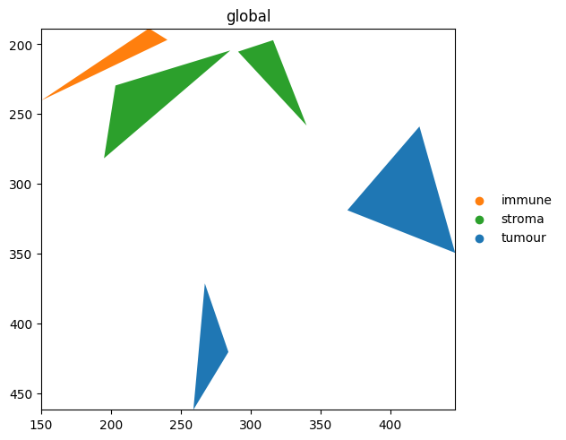
Because palette is a dict, the colour for 'tumour' is the same across every plot you reuse it in — handy for multi-panel figures.

make_palette_from_data currently supports shapes and points elements. For labels, set adata.uns['<col>_colors'] or pass palette=[...] directly to render_labels.

6. Which render_* accepts what

Function	palette	cmap	na_color
render_shapes	dict / list / str	yes	yes
render_points	dict / list / str	yes	yes
render_labels	dict / list / str	yes	yes
render_images	— (channels only)	yes	—

render_images colours pixels per channel, so palette and na_color don’t apply. Pass a list of cmaps via cmap=[...] to colour individual channels.

For reproducibility

# ruff: noqa: F401, F811, I001, E402
# fmt: off
import warnings
import dask
import spatialdata_plot

%load_ext watermark
# fmt: on

%watermark -v -m -p spatialdata,spatialdata_plot,matplotlib,numpy,pandas

Python implementation: CPython
Python version       : 3.13.7
IPython version      : 9.13.0

spatialdata     : 0.7.3
spatialdata_plot: 0.3.4
matplotlib      : 3.10.9
numpy           : 2.4.4
pandas          : 2.3.3

Compiler    : Clang 15.0.0 (clang-1500.1.0.2.5)
OS          : Darwin
Release     : 25.2.0
Machine     : arm64
Processor   : arm
CPU cores   : 8
Architecture: 64bit