Normalization and contrast in spatialdata-plot

This tutorial covers the norm= argument: how spatialdata-plot turns scalar data values into colors, and every knob you have to control contrast. By the end you should be able to:

• Explain what a norm does and when its limits are chosen for you.

• Set fixed contrast limits and choose how out-of-range values are drawn.

• Pick the right scaling — linear, logarithmic, power, or percentile — for your data.

• Give each image channel its own contrast, and use norm on shapes, points, and labels.

• Recognize the datashader caveat and the cases the renderer validates for you.

What a norm is

A norm is a matplotlib.colors.Normalize instance. It maps scalar data values → [0, 1] before the colormap turns them into colors, and it does two things:

1. Sets the contrast limits vmin / vmax — the data values that map to the bottom and top of the cmap.

2. Sets the scaling in between — linear, log, power, percentile-clipped — chosen by the subclass.

If you don’t pass a norm, you get a plain Normalize whose vmin/vmax are autoscaled to the data min/max. That is the default everywhere and it is unchanged.

The one rule: when vmin/vmax are unset, they autoscale from the data, and how they autoscale is decided by the norm subclass. spatialdata-plot delegates to each norm’s own logic, so every Normalize subclass works — including the percentile one below — with no special-casing.

Which renderers take norm

Renderer	norm accepts	Notes
render_images	a Normalize or a list[Normalize]	single = broadcast & autoscaled per channel; list = one per channel
render_shapes	a Normalize	scales a continuous color= column
render_points	a Normalize	continuous color=; resolved limits apply on the matplotlib backend
render_labels	a Normalize	scales a continuous color= column

Images are the only renderer that accepts a list, because an image has several channels that may each want their own contrast.

Setup

import matplotlib.pyplot as plt
import numpy as np
import spatialdata as sd
import spatialdata_plot as sdp  # noqa: F401  (registers the .pl accessor)
from matplotlib.colors import LogNorm, Normalize, PowerNorm, SymLogNorm
from spatialdata_plot import PercentileNormalize

sdata = sd.datasets.blobs()  # blobs_image has 3 channels: [0, 1, 2]
sdata

SpatialData object
├── Images
│     ├── 'blobs_image': DataArray[cyx] (3, 512, 512)
│     └── 'blobs_multiscale_image': DataTree[cyx] (3, 512, 512), (3, 256, 256), (3, 128, 128)
├── Labels
│     ├── 'blobs_labels': DataArray[yx] (512, 512)
│     └── 'blobs_multiscale_labels': DataTree[yx] (512, 512), (256, 256), (128, 128)
├── Points
│     └── 'blobs_points': DataFrame with shape: (<Delayed>, 4) (2D points)
├── Shapes
│     ├── 'blobs_circles': GeoDataFrame shape: (5, 2) (2D shapes)
│     ├── 'blobs_multipolygons': GeoDataFrame shape: (2, 1) (2D shapes)
│     └── 'blobs_polygons': GeoDataFrame shape: (5, 1) (2D shapes)
└── Tables
      └── 'table': AnnData (26, 3)
with coordinate systems:
    ▸ 'global', with elements:
        blobs_image (Images), blobs_multiscale_image (Images), blobs_labels (Labels), blobs_multiscale_labels (Labels), blobs_points (Points), blobs_circles (Shapes), blobs_multipolygons (Shapes), blobs_polygons (Shapes)

1. The default — per-channel min/max

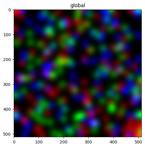
With no norm, every channel is scaled independently to its own min and max. This is the historical default.

blobs_image has three channels, so with the default colormap they are composited into a single RGB image — channel 0 → red, 1 → green, 2 → blue.

sdata.pl.render_images("blobs_image").pl.show()

2. Fixed contrast limits — Normalize(vmin, vmax)

Pin the window yourself. A single Normalize on a multi-channel image is broadcast to every channel. We render one channel with a colorbar so the limits are visible.

sdata.pl.render_images("blobs_image", channel=0, norm=Normalize(vmin=0.0, vmax=0.5), colorbar=True).pl.show()

3. Clipping — what happens outside [vmin, vmax]

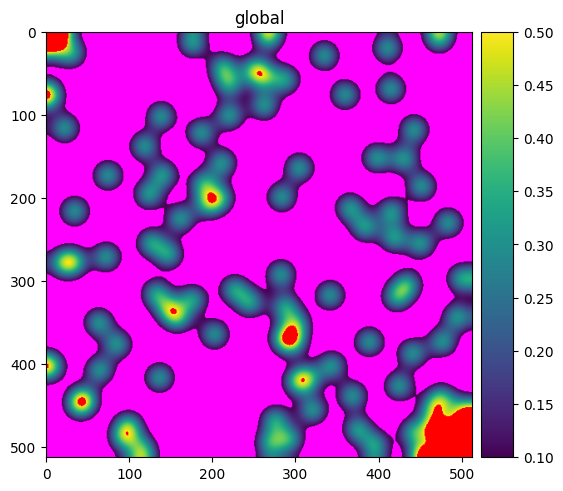
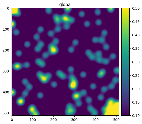
With clip=False (the default), values below vmin or above vmax are drawn in the colormap’s under/over colors (the special colors a colormap shows for values past each end, set via set_under / set_over). With clip=True, they are clamped to the ends instead. We use a cmap with distinct under/over colors to make the difference obvious.

First, clip=False — out-of-range pixels show magenta (under) and red (over):

cmap = plt.cm.viridis.copy()
cmap.set_under("magenta")
cmap.set_over("red")

sdata.pl.render_images("blobs_image", channel=0, cmap=cmap, norm=Normalize(0.1, 0.5, clip=False)).pl.show()

Now clip=True — the same out-of-range pixels are clamped to the cmap ends instead:

sdata.pl.render_images("blobs_image", channel=0, cmap=cmap, norm=Normalize(0.1, 0.5, clip=True)).pl.show()

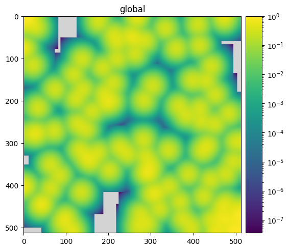
4. Logarithmic scaling — LogNorm

For data spanning orders of magnitude. On the non-image renderers (shapes, points, labels), spatialdata-plot resolves LogNorm limits from the strictly-positive data and falls back to a valid domain when none exist, so a non-positive vmin never raises a late “Invalid vmin or vmax”. On images, as below, LogNorm is applied directly by matplotlib.

sdata.pl.render_images("blobs_image", channel=0, norm=LogNorm(), colorbar=True).pl.show()

5. Other matplotlib norms work too

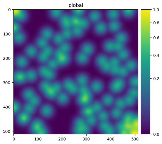
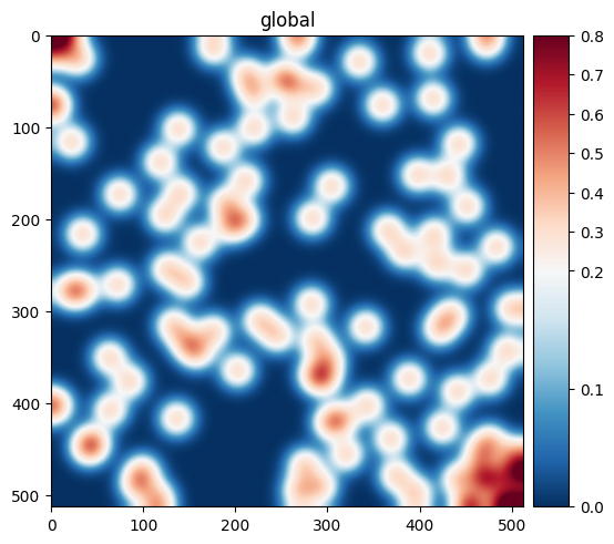
Because the limits come from each norm’s own logic, any Normalize subclass plugs in. Two common ones: PowerNorm (gamma correction) and SymLogNorm (log scaling with a linear region around zero).

sdata.pl.render_images("blobs_image", channel=0, norm=PowerNorm(gamma=0.5), colorbar=True).pl.show()

sdata.pl.render_images("blobs_image", channel=0, norm=SymLogNorm(linthresh=0.05), colorbar=True).pl.show()

6. Percentile contrast — PercentileNormalize

Heavy-tailed images (fluorescence, Xenium morphology) often look dim: a single bright outlier sets the min/max vmax and crushes the rest of the signal to near-black. PercentileNormalize(pmin, pmax) derives the limits from data percentiles instead — the same idea as the contrast sliders in viewers like Xenium Explorer.

• pmin/pmax are validated to satisfy 0 <= pmin < pmax <= 100.

• NaN / inf / masked pixels are excluded from the percentile computation.

• A single instance is autoscaled independently per channel.

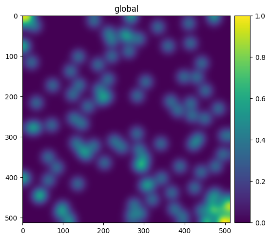
Here is the default min/max rendering of one channel:

sdata.pl.render_images("blobs_image", channel=0).pl.show()

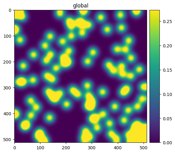
And the same channel with the top 10% of values clipped, lifting the bulk of the signal:

sdata.pl.render_images("blobs_image", channel=0, norm=PercentileNormalize(0, 90)).pl.show()

7. Per-channel norms for images

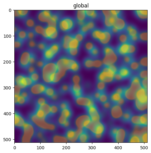
Pass a list of norms, one per channel (its length must equal the number of channels). You can mix subclasses freely — give each channel exactly the contrast it needs.

norms = [PercentileNormalize(0, 99), PercentileNormalize(0, 90), PercentileNormalize(0, 80)]
sdata.pl.render_images("blobs_image", channel=[0, 1, 2], norm=norms).pl.show()

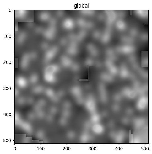
mixed = [Normalize(0, 0.5), LogNorm(), PercentileNormalize(2, 98)]
sdata.pl.render_images("blobs_image", channel=[0, 1, 2], norm=mixed, cmap=[plt.cm.gray] * 3).pl.show()

WARNING  render_images: You're blending multiple cmaps. If the plot doesn't look like you expect, it might be      
         because your cmaps go from a given color to 'white', and not to 'transparent'. Therefore, the 'white' of  
         higher layers will overlay the lower layers. Consider using 'palette' instead.

8. Combining with transfunc

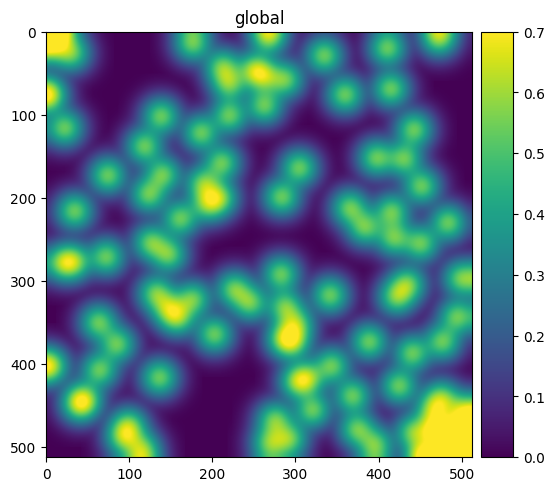
transfunc transforms the raw array first, then norm scales the result. So transfunc=np.sqrt with a norm operates on the square-rooted data — handy for pairing a fixed transform with explicit limits.

sdata.pl.render_images("blobs_image", channel=0, transfunc=np.sqrt, norm=Normalize(0.0, 0.7), colorbar=True).pl.show()

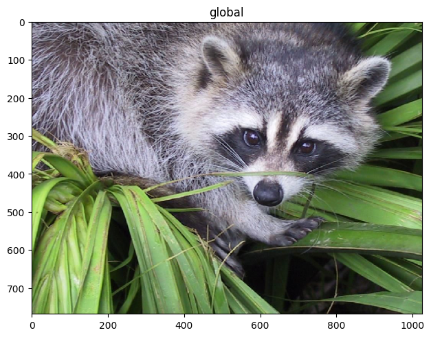
9. True RGB images

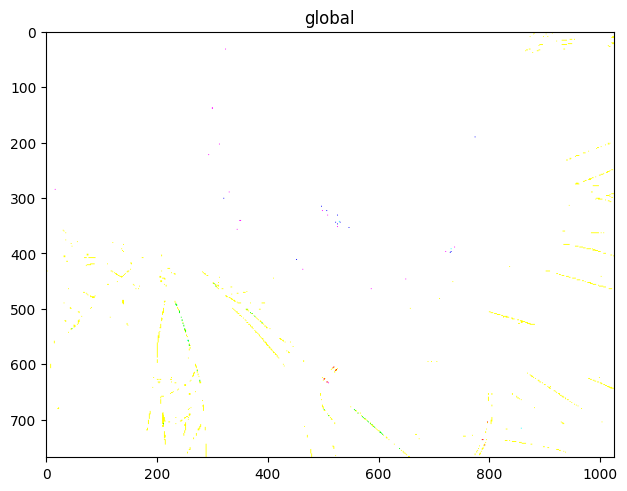
When the channels are literally named {r, g, b(, a)}, the RGB path composites them with one shared scale to preserve hue balance. If you pass a norm with explicit vmin/vmax, it is applied per channel and clipped to [0, 1]; otherwise channels are scaled by their dtype.

rac = sd.datasets.raccoon()  # a real RGB photo
rac.pl.render_images("raccoon").pl.show()

rac.pl.render_images("raccoon", norm=Normalize(0.0, 0.5, clip=True)).pl.show()

10. Norms on shapes, points, and labels

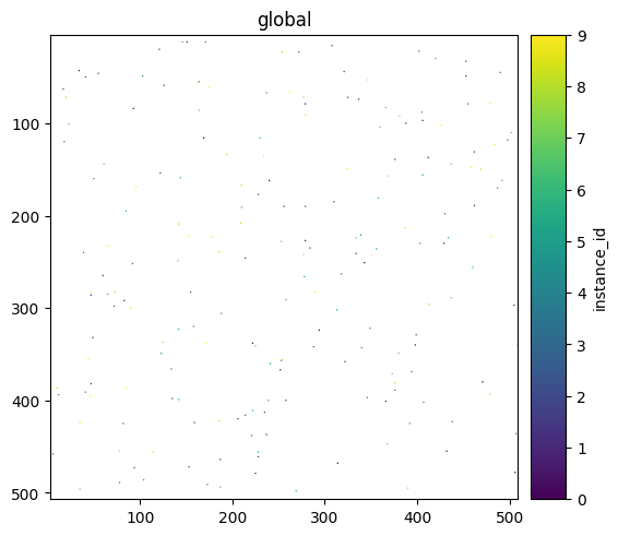
For non-image renderers, norm scales a continuous color= column. The same resolved norm drives both the fill colors and the colorbar, so the bar always matches the pixels — a LogNorm colorbar stays logarithmic.

Shapes, colored by a continuous geometry column:

sdata.pl.render_shapes("blobs_circles", color="radius", norm=Normalize(), colorbar=True).pl.show()

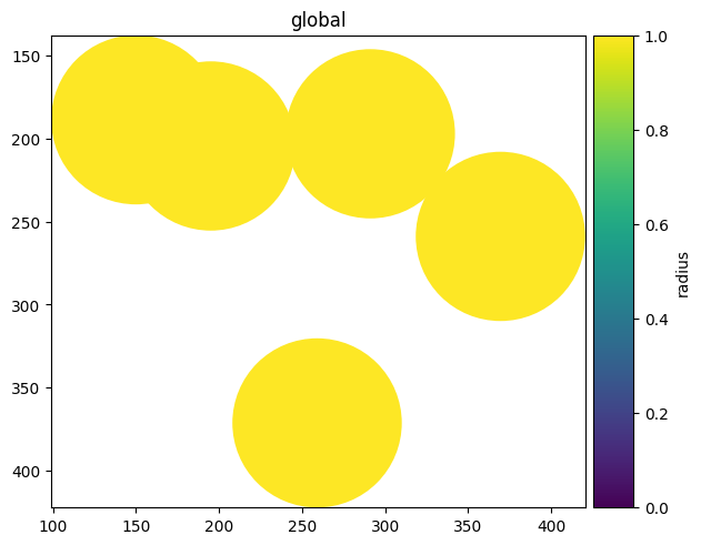
sdata.pl.render_shapes("blobs_circles", color="radius", norm=PercentileNormalize(5, 95), colorbar=True).pl.show()

Points, colored by a continuous column:

sdata.pl.render_points("blobs_points", color="instance_id", norm=Normalize(), colorbar=True).pl.show()

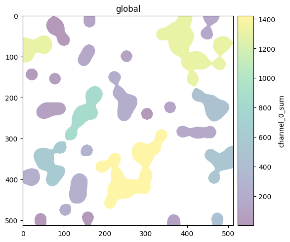
Labels, colored by a continuous table column:

sdata.pl.render_labels("blobs_labels", color="channel_0_sum", norm=PercentileNormalize(2, 98), colorbar=True).pl.show()

11. The datashader caveat

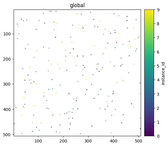
On the datashader backend, contrast autoscales to the aggregated value range, not to a norm’s percentiles. Explicit vmin/vmax are still honored. For percentile-driven contrast on points, use the default matplotlib backend.

The cell below passes PercentileNormalize(5, 95), but on datashader those percentile limits are ignored — the contrast follows the aggregate range instead.

sdata.pl.render_points("blobs_points", color="instance_id", method="datashader", norm=PercentileNormalize(5, 95)).pl.show()

12. Edge cases the renderer handles for you

The renderer validates norm inputs up front and fails with an actionable message rather than deep inside matplotlib.

A per-channel norm list of the wrong length is rejected with a clear message:

try:
    sdata.pl.render_images("blobs_image", channel=[0, 1, 2], norm=[Normalize(0, 1)] * 2, cmap=[plt.cm.gray] * 3).pl.show()
except ValueError as e:
    print("ValueError:", e)

ValueError: Length of 'norm' list (2) must match the number of channels (3).

And invalid percentile bounds are caught at construction time:

for bad in [(50, 50), (90, 10), (-1, 50), (0, 101)]:
    try:
        PercentileNormalize(*bad)
    except ValueError as e:
        print(f"PercentileNormalize{bad} -> {e}")

PercentileNormalize(50, 50) -> Require 0 <= pmin < pmax <= 100, got pmin=50, pmax=50.
PercentileNormalize(90, 10) -> Require 0 <= pmin < pmax <= 100, got pmin=90, pmax=10.
PercentileNormalize(-1, 50) -> Require 0 <= pmin < pmax <= 100, got pmin=-1, pmax=50.
PercentileNormalize(0, 101) -> Require 0 <= pmin < pmax <= 100, got pmin=0, pmax=101.

Summary

• norm is a matplotlib Normalize; the default is per-channel min/max and is unchanged.

• Limits come from each norm’s own logic, so Normalize, LogNorm, PowerNorm, SymLogNorm, and PercentileNormalize all just work.

• PercentileNormalize(pmin, pmax) fixes heavy-tailed dimness with no new parameter — it’s opt-in.

• Only render_images accepts a list of norms (one per channel); single instances broadcast.

• The colorbar always reflects the resolved norm; datashader autoscales to the aggregate.