Cropping a plot with crop_coord

Most spatial datasets are far larger than the region you want to look at. crop_coord restricts a plot to a bounding box at draw time: the SpatialData object is untouched, only the window is rendered — and for images and labels only the window is ever rasterized, so zooming into a gigapixel slide costs about as much as plotting a thumbnail.

This tutorial uses the Xenium cells dataset from squidpy.datasets (a 550 × 450 µm section with a four-channel fluorescence image, cell and nucleus segmentations, transcripts and a cell table).

Setup

import warnings

import matplotlib.pyplot as plt
import squidpy as sq
from matplotlib.patches import Rectangle

import spatialdata as sd
import spatialdata_plot  # noqa: F401  # registers the .pl accessor
from spatialdata_plot import PercentileNormalize

warnings.filterwarnings("ignore")

sdata = sq.datasets.cells()
sdata

INFO     Loading existing dataset from data/spatialdata/cells.zarr

SpatialData object, with associated Zarr store: /Users/tim.treis/Documents/GitHub/spatialdata-plot-notebooks/tutorials/data/spatialdata/cells.zarr
├── Images
│     ├── 'he_aligned': DataTree[cyx] (3, 430, 540), (3, 215, 270)
│     ├── 'he_image': DataTree[cyx] (3, 423, 339), (3, 211, 169)
│     └── 'morphology_focus': DataTree[cyx] (4, 430, 540), (4, 215, 270)
├── Labels
│     ├── 'cell_labels': DataTree[yx] (430, 540), (215, 270)
│     ├── 'nucleus_labels': DataTree[yx] (430, 540), (215, 270)
│     └── 'tissue_labels': DataTree[yx] (430, 540), (215, 270)
├── Points
│     └── 'transcripts': DataFrame with shape: (<Delayed>, 13) (3D points)
├── Shapes
│     ├── 'cell_boundaries': GeoDataFrame shape: (94, 1) (2D shapes)
│     └── 'nucleus_boundaries': GeoDataFrame shape: (94, 2) (2D shapes)
└── Tables
      └── 'table': AnnData (94, 5101)
with coordinate systems:
    ▸ 'global', with elements:
        he_aligned (Images), he_image (Images), morphology_focus (Images), cell_labels (Labels), nucleus_labels (Labels), tissue_labels (Labels), transcripts (Points), cell_boundaries (Shapes), nucleus_boundaries (Shapes)

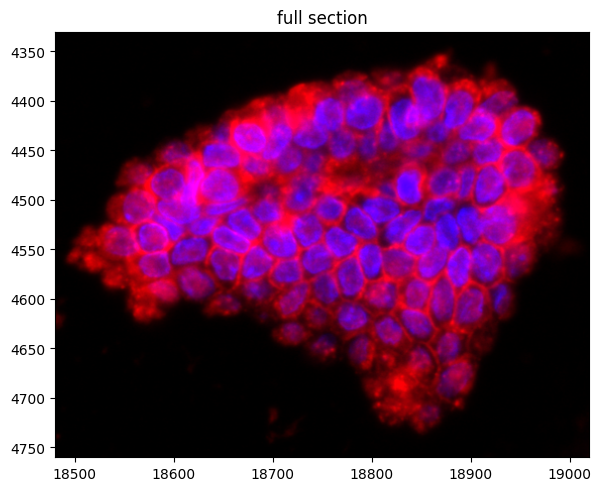
We render the DAPI (nuclei) and membrane channels of morphology_focus throughout, so we bundle those arguments once. See the Multichannel & fluorescence images tutorial for what they do.

IMG = dict(
    channel=["DAPI", "ATP1A1/CD45/E-Cadherin"],
    palette=["blue", "red"],
    norm=[PercentileNormalize(1, 99)] * 2,
)
sdata.pl.render_images("morphology_focus", **IMG).pl.show(title="full section")

1. Zooming in — crop_coord

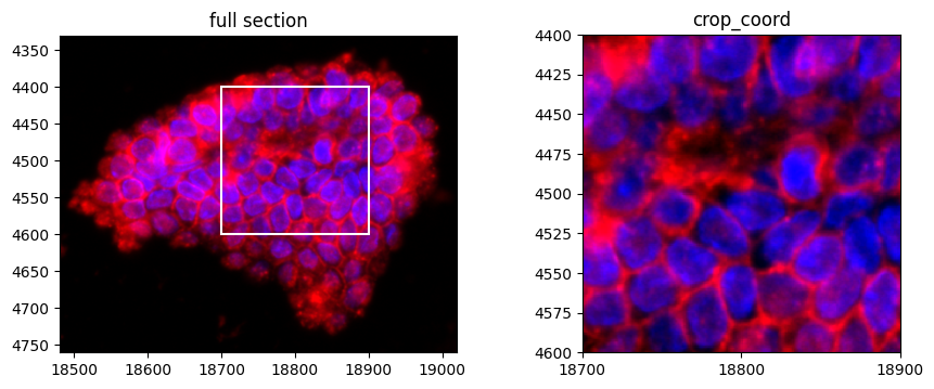
crop_coord is a tuple (xmin, xmax, ymin, ymax) in the units of the rendered coordinate system — the same order as ax.axis(...) and as crop_coord in scanpy.pl.spatial / squidpy.pl.spatial_scatter. Here the units are microns; we zoom into a 200 × 200 µm window. The white box is a plain matplotlib Rectangle, drawn so you can see where the crop sits.

CROP = (18700, 18900, 4400, 4600)  # xmin, xmax, ymin, ymax in µm


def crop_box(crop, **style):
    xmin, xmax, ymin, ymax = crop
    return Rectangle((xmin, ymin), xmax - xmin, ymax - ymin, fill=False, edgecolor="white", **style)


fig, (ax_full, ax_crop) = plt.subplots(1, 2, figsize=(10, 4.5), gridspec_kw={"width_ratios": [1.25, 1]})
sdata.pl.render_images("morphology_focus", **IMG).pl.show(ax=ax_full, title="full section")
ax_full.add_patch(crop_box(CROP, lw=1.5))
sdata.pl.render_images("morphology_focus", **IMG).pl.show(ax=ax_crop, crop_coord=CROP, title="crop_coord")
ax_crop.set_xticks([18700, 18800, 18900])
fig.subplots_adjust(wspace=0.35)

2. One window for every layer

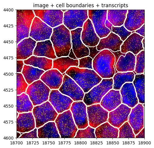
crop_coord is a show() argument, so it applies to every render_* call in the chain. Points and shapes are subsetted to the window before drawing; images and labels are rasterized for the window only.

(
    sdata.pl.render_images("morphology_focus", **IMG)
    .pl.render_shapes("cell_boundaries", fill_alpha=0, outline=True, outline_color="white")
    .pl.render_points("transcripts", color="yellow", size=1)
    .pl.show(crop_coord=CROP, title="image + cell boundaries + transcripts")
)

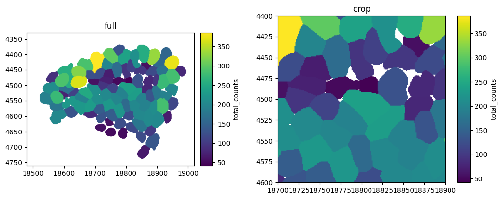
3. Keeping colours comparable

Cropping changes what the auto-scaled colour ranges see:

• Points, shapes and labels keep the range of the full element, so a colour in the crop means the same thing as in the uncropped plot — note the identical colorbars below.

• Images are contrast-stretched over the window, because only the window is ever read. A crop of a dim region therefore looks brighter than the same region in the full plot.

fig, axes = plt.subplots(1, 2, figsize=(11, 5))
sdata.pl.render_labels("cell_labels", color="total_counts", fill_alpha=1).pl.show(ax=axes[0], title="full")
sdata.pl.render_labels("cell_labels", color="total_counts", fill_alpha=1).pl.show(
    ax=axes[1], crop_coord=CROP, title="crop"
)
fig.subplots_adjust(wspace=0.5)

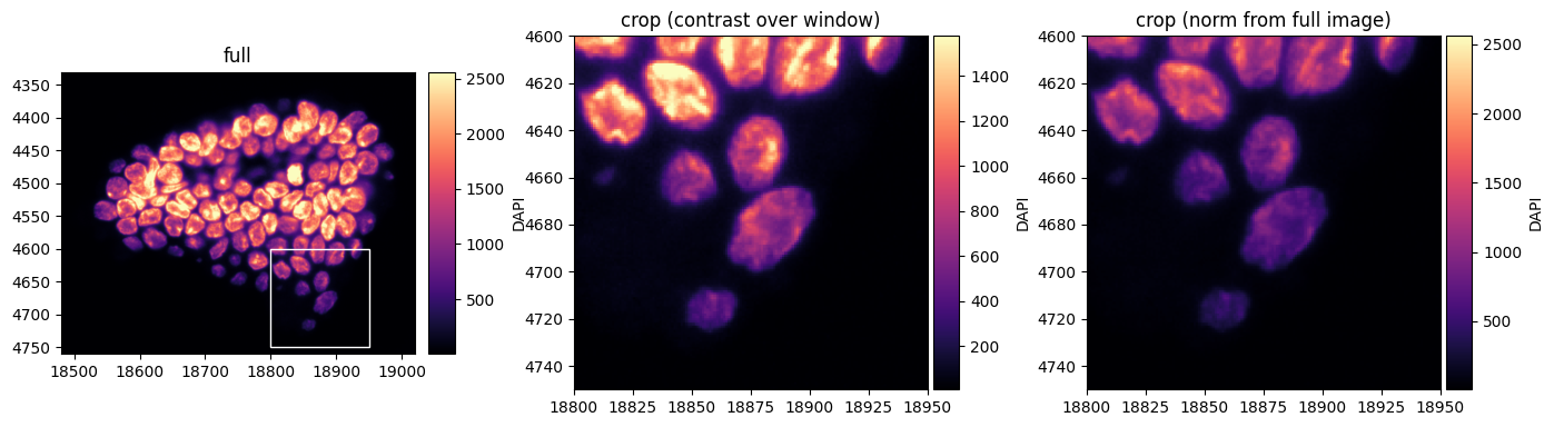
The effect is easiest to see on a dim region: the lobe at the bottom right is roughly half as bright as the brightest nuclei, so cropped on its own it gets stretched to full contrast. To pin image contrast to the full-image range, pass explicit limits — a norm (or vmin/vmax). Here we take the 1st and 99th percentile of the full DAPI channel:

from matplotlib.colors import Normalize

DIM = (18800, 18950, 4600, 4750)  # a dim window at the bottom right

dapi = sdata["morphology_focus"]["scale0"].image.sel(c="DAPI")
fixed = Normalize(*dapi.quantile([0.01, 0.99]).values)

fig, axes = plt.subplots(1, 3, figsize=(16, 5))
sdata.pl.render_images("morphology_focus", channel="DAPI", cmap="magma", norm=PercentileNormalize(1, 99)).pl.show(
    ax=axes[0], title="full"
)
axes[0].add_patch(crop_box(DIM))
sdata.pl.render_images("morphology_focus", channel="DAPI", cmap="magma", norm=PercentileNormalize(1, 99)).pl.show(
    ax=axes[1], crop_coord=DIM, title="crop (contrast over window)"
)
sdata.pl.render_images("morphology_focus", channel="DAPI", cmap="magma", norm=fixed).pl.show(
    ax=axes[2], crop_coord=DIM, title="crop (norm from full image)"
)
fig.subplots_adjust(wspace=0.45)

4. crop_coord vs bounding_box_query

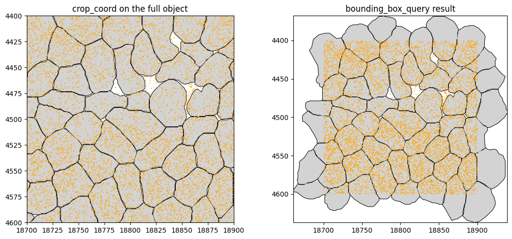
spatialdata.bounding_box_query builds a new SpatialData object containing only the elements inside the box. crop_coord changes only what is drawn. The pictures are the same; the difference is what you are left with:

• use crop_coord to look at a region — nothing is copied, and images stay lazy;

• use bounding_box_query when you need the subset as data — to count, analyse, or save it.

Note the axes: crop_coord pins the view to the box, whereas the query keeps every cell that intersects the box in full, so its result spills over the edges.

subset = sd.bounding_box_query(
    sdata,
    axes=("x", "y"),
    min_coordinate=[CROP[0], CROP[2]],
    max_coordinate=[CROP[1], CROP[3]],
    target_coordinate_system="global",
)
print(f"cells: {len(sdata['cell_boundaries'])} in the full object, {len(subset['cell_boundaries'])} in the query result")
print(f"transcripts: {len(sdata['transcripts'])} in the full object, {len(subset['transcripts'])} in the query result")

fig, axes = plt.subplots(1, 2, figsize=(11, 5))
sdata.pl.render_shapes("cell_boundaries", color="lightgray", outline=True).pl.render_points(
    "transcripts", color="orange", size=2
).pl.show(ax=axes[0], crop_coord=CROP, title="crop_coord on the full object")
subset.pl.render_shapes("cell_boundaries", color="lightgray", outline=True).pl.render_points(
    "transcripts", color="orange", size=2
).pl.show(ax=axes[1], title="bounding_box_query result")
fig.tight_layout()

cells: 94 in the full object, 55 in the query result
transcripts: 19479 in the full object, 7466 in the query result

5. One coordinate system at a time

The box is expressed in one coordinate system’s units, so crop_coord requires a single coordinate system to be rendered. If your object has several, pick one with coordinate_systems="global" (or whichever applies) in the same show() call.

For reproducibility

# ruff: noqa: F401, F811, I001, E402
# fmt: off
import spatialdata_plot

%load_ext watermark
# fmt: on

%watermark -v -m -p spatialdata,spatialdata_plot,squidpy,matplotlib,numpy

Python implementation: CPython
Python version       : 3.14.4
IPython version      : 9.13.0

spatialdata     : 0.7.3
spatialdata_plot: 0.4.2
squidpy         : 1.8.3
matplotlib      : 3.10.9
numpy           : 2.4.4

Compiler    : Clang 20.1.8 
OS          : Darwin
Release     : 25.2.0
Machine     : arm64
Processor   : arm
CPU cores   : 8
Architecture: 64bit