Styling shapes and labels in spatialdata-plot

color= decides what colour a shape or label gets; a separate set of arguments decides how it is drawn — how opaque the fill is, whether there is an outline, and how thick and what colour that outline is. This tutorial walks through those styling knobs for render_shapes and render_labels. By the end you should be able to:

• Control fill opacity with fill_alpha.

• Turn outlines on and style their width, colour, and opacity.

• Draw a double outline (outer + inner).

• Draw hollow shapes (outline only) and translucent label masks over an image.

• Trace segmentation boundaries with outline and contour_px on labels.

We use the synthetic blobs dataset throughout so the notebook stays small and reproducible.

Setup

import spatialdata as sd
import spatialdata_plot  # noqa: F401  # registers the .pl accessor

sdata = sd.datasets.blobs()
sdata

SpatialData object
├── Images
│     ├── 'blobs_image': DataArray[cyx] (3, 512, 512)
│     └── 'blobs_multiscale_image': DataTree[cyx] (3, 512, 512), (3, 256, 256), (3, 128, 128)
├── Labels
│     ├── 'blobs_labels': DataArray[yx] (512, 512)
│     └── 'blobs_multiscale_labels': DataTree[yx] (512, 512), (256, 256), (128, 128)
├── Points
│     └── 'blobs_points': DataFrame with shape: (<Delayed>, 4) (2D points)
├── Shapes
│     ├── 'blobs_circles': GeoDataFrame shape: (5, 2) (2D shapes)
│     ├── 'blobs_multipolygons': GeoDataFrame shape: (2, 1) (2D shapes)
│     └── 'blobs_polygons': GeoDataFrame shape: (5, 1) (2D shapes)
└── Tables
      └── 'table': AnnData (26, 3)
with coordinate systems:
    ▸ 'global', with elements:
        blobs_image (Images), blobs_multiscale_image (Images), blobs_labels (Labels), blobs_multiscale_labels (Labels), blobs_points (Points), blobs_circles (Shapes), blobs_multipolygons (Shapes), blobs_polygons (Shapes)

1. Default shapes

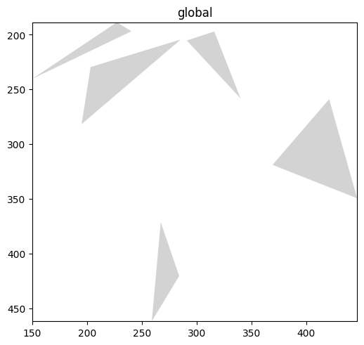
The element names used below (blobs_polygons, blobs_labels, blobs_image) are the keys shown in the sdata repr above. By default, shapes are drawn as filled patches with no outline. We start from blobs_polygons.

sdata.pl.render_shapes('blobs_polygons').pl.show()

2. Fill opacity — fill_alpha

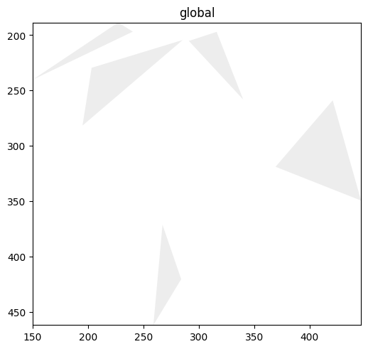
fill_alpha sets how opaque the fill is, from 1.0 (solid) down to 0.0 (invisible). Lower it when shapes overlap or sit on top of an image you still want to see.

sdata.pl.render_shapes('blobs_polygons', fill_alpha=0.4).pl.show()

3. Outlines — the outline toggle

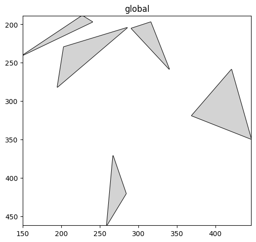
Pass outline=True to draw a border around each shape. Outlines are off by default; turning the toggle on gives every shape a crisp edge. (Leaving outline=None — the default — instead infers the border from whether you set any outline_* argument.)

sdata.pl.render_shapes('blobs_polygons', outline=True).pl.show()

4. Styling the outline — width, colour, opacity

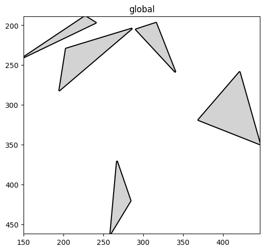
outline_width, outline_color, and outline_alpha control the border once outline=True.

sdata.pl.render_shapes(
    'blobs_polygons',
    outline=True,
    outline_width=3.0,
    outline_color='black',
    outline_alpha=1.0,
).pl.show()

5. Two outlines — outer and inner

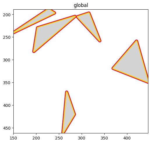
outline_width, outline_color, and outline_alpha each accept a two-tuple to draw two concentric borders — an outer band and an inner one — in a single call. Each tuple is (outer, inner). Useful for a border that reads against both light and dark backgrounds, or simply to make an edge pop. Give any one of them a tuple and the others fall back to per-band defaults (widths 1.5/0.5, colours #000000/#ffffff for outer/inner).

sdata.pl.render_shapes(
    'blobs_polygons',
    outline=True,
    outline_width=(8.0, 4.0),          # (outer, inner)
    outline_color=('crimson', 'gold'),
    outline_alpha=(1.0, 1.0),
).pl.show()

6. Hollow shapes — outline only

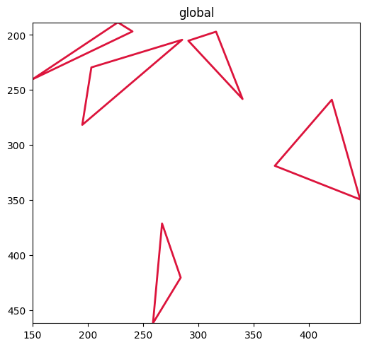
Combine a transparent fill (fill_alpha=0.0) with an outline to get outline-only shapes — useful for marking regions of interest without hiding what is underneath.

sdata.pl.render_shapes(
    'blobs_polygons',
    fill_alpha=0.0,
    outline=True,
    outline_width=2.0,
    outline_color='crimson',
).pl.show()

7. Resizing geometries — scale

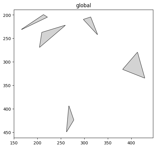
scale multiplies each shape’s size about its centroid: shrink to separate crowded shapes, or grow to emphasise them. Here the polygons are drawn at 60% size with an outline.

sdata.pl.render_shapes('blobs_polygons', scale=0.6, outline=True).pl.show()

8. Labels use the same vocabulary

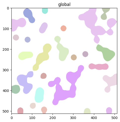
Label (segmentation-mask) rendering shares the fill/outline arguments. By default, masks are drawn semi-transparent (fill_alpha=0.4), not solid — so anything layered beneath them still shows through.

sdata.pl.render_labels('blobs_labels').pl.show()

9. Translucent masks over an image — fill_alpha

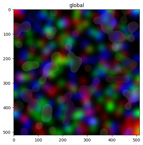
Lowering fill_alpha below its 0.4 default lets more of the underlying image show through — the standard way to overlay a segmentation on the raw data. We layer the labels on top of blobs_image.

(
    sdata.pl.render_images('blobs_image')
    .pl.render_labels('blobs_labels', fill_alpha=0.2)
).pl.show()

10. Segmentation boundaries — outline and contour_px

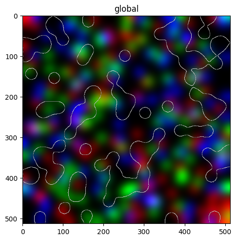
For labels, outline=True traces each mask’s boundary. contour_px sets the boundary thickness in pixels, and outline_color/outline_alpha style it. Set fill_alpha=0.0 to show the boundaries alone.

(
    sdata.pl.render_images('blobs_image')
    .pl.render_labels(
        'blobs_labels',
        fill_alpha=0.0,
        outline=True,
        contour_px=3,
        outline_color='white',
    )
).pl.show()

11. Putting it together

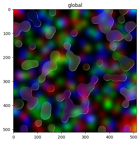
A translucent fill plus a crisp boundary over the image gives a readable segmentation overlay — the combination you will reach for most often.

(
    sdata.pl.render_images('blobs_image')
    .pl.render_labels(
        'blobs_labels',
        fill_alpha=0.3,
        outline=True,
        contour_px=2,
        outline_color='white',
        outline_alpha=1.0,
    )
).pl.show()

Summary

• fill_alpha sets fill opacity for both shapes and labels.

• outline=True adds a border for shapes and labels; style it with outline_width, outline_color, and outline_alpha, and for labels set the boundary thickness with contour_px.

• Pass a two-tuple to outline_width/outline_color/outline_alpha for a double outline (outer + inner).

• outline_color also accepts a column name when the element is annotated by a table, colouring each border per shape — see the Colouring tutorial.

• A transparent fill plus an outline gives hollow shapes or boundary-only segmentation overlays.

• scale resizes shape geometries about their centroids.

For reproducibility

# ruff: noqa: F401, F811, I001, E402
# fmt: off
import warnings
import spatialdata_plot

%load_ext watermark
# fmt: on

%watermark -v -m -p spatialdata,spatialdata_plot,matplotlib,numpy,pandas

Python implementation: CPython
Python version       : 3.14.4
IPython version      : 9.13.0

spatialdata     : 0.7.3
spatialdata_plot: 0.4.2
matplotlib      : 3.10.9
numpy           : 2.4.4
pandas          : 2.3.3

Compiler    : Clang 20.1.8 
OS          : Darwin
Release     : 25.2.0
Machine     : arm64
Processor   : arm
CPU cores   : 8
Architecture: 64bit