Multi-panel colouring in spatialdata-plot

Passing a list to color= renders one panel per colouring in a single figure, the same way scanpy’s color=[...] works. By the end you should be able to:

• Turn a single render_labels/render_shapes call into a grid of panels.

• Mix categorical and continuous colourings in one figure, each with its own legend or colourbar.

• Control the grid width with show(ncols=...) and share palette/cmap across panels.

We use the synthetic blobs dataset throughout so the notebook stays small and reproducible.

Setup

import numpy as np
import pandas as pd

import spatialdata as sd
import spatialdata_plot  # noqa: F401  # registers the .pl accessor

sdata = sd.datasets.blobs()

rng = np.random.default_rng(0)

# A categorical and (built-in) continuous columns on the table annotate blobs_labels.
table = sdata.tables['table']
table.obs['cell_type'] = pd.Categorical(
    rng.choice(['A', 'B', 'C', 'D', 'E'], size=table.n_obs),
    categories=['A', 'B', 'C', 'D', 'E'],
)

# A categorical and a continuous column directly on a shapes GeoDataFrame.
sdata.shapes['blobs_polygons']['region_type'] = pd.Categorical(
    ['stroma', 'tumour', 'stroma', 'immune', 'tumour'],
)
sdata.shapes['blobs_polygons']['score'] = rng.random(len(sdata.shapes['blobs_polygons']))
sdata

SpatialData object
├── Images
│     ├── 'blobs_image': DataArray[cyx] (3, 512, 512)
│     └── 'blobs_multiscale_image': DataTree[cyx] (3, 512, 512), (3, 256, 256), (3, 128, 128)
├── Labels
│     ├── 'blobs_labels': DataArray[yx] (512, 512)
│     └── 'blobs_multiscale_labels': DataTree[yx] (512, 512), (256, 256), (128, 128)
├── Points
│     └── 'blobs_points': DataFrame with shape: (<Delayed>, 4) (2D points)
├── Shapes
│     ├── 'blobs_circles': GeoDataFrame shape: (5, 2) (2D shapes)
│     ├── 'blobs_multipolygons': GeoDataFrame shape: (2, 1) (2D shapes)
│     └── 'blobs_polygons': GeoDataFrame shape: (5, 3) (2D shapes)
└── Tables
      └── 'table': AnnData (26, 3)
with coordinate systems:
    ▸ 'global', with elements:
        blobs_image (Images), blobs_multiscale_image (Images), blobs_labels (Labels), blobs_multiscale_labels (Labels), blobs_points (Points), blobs_circles (Shapes), blobs_multipolygons (Shapes), blobs_polygons (Shapes)

1. From one colouring to many

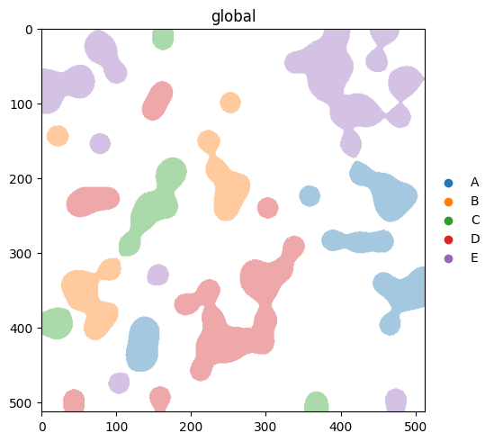
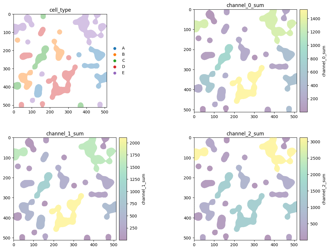
A single string colours one panel. Pass a list and each entry becomes its own panel of the same element — one figure, many colourings. show(ncols=...) lays the panels out in a grid.

sdata.pl.render_labels('blobs_labels', color='cell_type').pl.show()

# Four colourings of the same labels, arranged 2x2.
sdata.pl.render_labels(
    'blobs_labels',
    color=['cell_type', 'channel_0_sum', 'channel_1_sum', 'channel_2_sum'],
).pl.show(ncols=2)

2. Mixing categorical and continuous

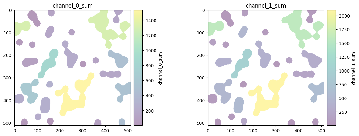
The panels above already mix a categorical colouring (cell_type, drawn with a legend) with continuous ones (the channel sums, drawn with colourbars). Each panel auto-scales independently, so a channel with a small dynamic range still uses the full colourmap rather than being flattened against a brighter channel.

sdata.pl.render_labels(
    'blobs_labels',
    color=['channel_0_sum', 'channel_1_sum'],
).pl.show()

3. Multi-panel render_shapes

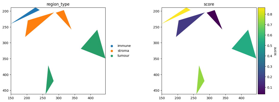
The list form works identically for shapes. Here a categorical (region_type) and a continuous column (score) on the same polygons render side by side.

sdata.pl.render_shapes(
    'blobs_polygons',
    color=['region_type', 'score'],
).pl.show()

4. Controlling the grid with ncols

ncols sets how many panels sit in a row; the rest wrap onto new rows. The same four colourings become a single row with ncols=4 or a 2x2 grid with ncols=2.

sdata.pl.render_labels(
    'blobs_labels',
    color=['cell_type', 'channel_0_sum', 'channel_1_sum', 'channel_2_sum'],
).pl.show(ncols=4)

5. Shared palette / cmap / norm across panels

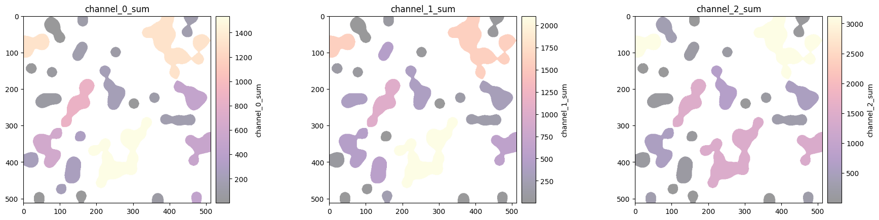
palette, cmap, norm and groups are applied to every panel, so a single keyword styles the whole figure. Autoscaling still happens per panel unless you pin it with an explicit norm.

sdata.pl.render_labels(
    'blobs_labels',
    color=['channel_0_sum', 'channel_1_sum', 'channel_2_sum'],
    cmap='magma',
).pl.show(ncols=3)

For reproducibility

# ruff: noqa: F401, F811, I001, E402
# fmt: off
import warnings
import dask
import spatialdata_plot

%load_ext watermark
# fmt: on

%watermark -v -m -p spatialdata,spatialdata_plot,matplotlib,numpy,pandas

Python implementation: CPython
Python version       : 3.14.4
IPython version      : 9.13.0

spatialdata     : 0.7.3
spatialdata_plot: 0.4.1
matplotlib      : 3.10.9
numpy           : 2.4.4
pandas          : 2.3.3

Compiler    : Clang 20.1.8 
OS          : Darwin
Release     : 25.2.0
Machine     : arm64
Processor   : arm
CPU cores   : 8
Architecture: 64bit