Scalebars in spatialdata-plot

A scalebar tells the reader the physical size of what they are looking at. spatialdata-plot draws one through the scalebar_* arguments of .pl.show(). The one thing to get right is scalebar_dx: because SpatialData coordinate systems carry no physical-unit metadata, you have to tell the plot how large one axes-unit is.

By the end you should be able to:

• Add a scalebar and explain what scalebar_dx means and why it is required.

• Choose the unit with scalebar_units and let the bar auto-scale (µm → mm).

• Style the bar (placement, colour, box, length, fonts) via scalebar_params.

• Pin an exact bar length with fixed_value.

We use the synthetic blobs dataset throughout so the notebook stays small and reproducible. Its images have no real-world scale, so we will pretend they were acquired at 0.5 µm per pixel.

Setup

import spatialdata as sd
import spatialdata_plot  # noqa: F401  # registers the .pl accessor

sdata = sd.datasets.blobs()
sdata

SpatialData object
├── Images
│     ├── 'blobs_image': DataArray[cyx] (3, 512, 512)
│     └── 'blobs_multiscale_image': DataTree[cyx] (3, 512, 512), (3, 256, 256), (3, 128, 128)
├── Labels
│     ├── 'blobs_labels': DataArray[yx] (512, 512)
│     └── 'blobs_multiscale_labels': DataTree[yx] (512, 512), (256, 256), (128, 128)
├── Points
│     └── 'blobs_points': DataFrame with shape: (<Delayed>, 4) (2D points)
├── Shapes
│     ├── 'blobs_circles': GeoDataFrame shape: (5, 2) (2D shapes)
│     ├── 'blobs_multipolygons': GeoDataFrame shape: (2, 1) (2D shapes)
│     └── 'blobs_polygons': GeoDataFrame shape: (5, 1) (2D shapes)
└── Tables
      └── 'table': AnnData (26, 3)
with coordinate systems:
    ▸ 'global', with elements:
        blobs_image (Images), blobs_multiscale_image (Images), blobs_labels (Labels), blobs_multiscale_labels (Labels), blobs_points (Points), blobs_circles (Shapes), blobs_multipolygons (Shapes), blobs_polygons (Shapes)

1. The one required piece: scalebar_dx

scalebar_dx is the physical size of one axes-unit. The blobs image is indexed in pixels, so one axes-unit is one pixel; at our assumed resolution that is 0.5 µm. Pass that as scalebar_dx, and the unit it is measured in as scalebar_units. Note that scalebar_dx should be a float.

PX_SIZE_UM = 0.5  # physical size of one pixel, taken from the acquisition metadata

sdata.pl.render_images("blobs_image").pl.show(
    scalebar_dx=PX_SIZE_UM,
    scalebar_units="um",
)

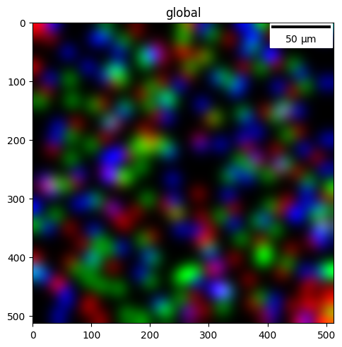
Without scalebar_dx there is no scalebar — the plot has no way to know the physical size, and it never guesses. Two things worth remembering:

• If your coordinate system is in pixels, scalebar_dx is the micron-per-pixel value.

• If a transformation already put the coordinate system in physical units (µm), then one axes-unit is one µm, so scalebar_dx=1.0.

In multi-panel plots the same scalebar is drawn on every panel.

2. Units and auto-scaling

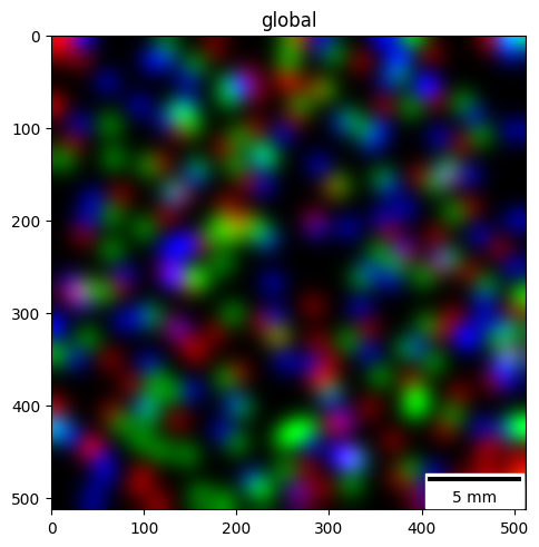
scalebar_units is simply the unit your scalebar_dx is expressed in. matplotlib-scalebar then picks a human-friendly magnitude automatically: a bar spanning thousands of µm is shown in mm. The same image at a coarse 50 µm/pixel gives a bar labelled in mm:

sdata.pl.render_images("blobs_image").pl.show(
    scalebar_dx=50.0,  # coarse resolution: 50 µm per pixel
    scalebar_units="um",
    scalebar_params={"location": "lower right"},
)

3. Placement and appearance with scalebar_params

scalebar_params is a dict forwarded verbatim to matplotlib-scalebar’s ScaleBar, so every option it supports is available. The ones you will reach for most:

• location — which corner ("lower right", "upper left", …).

• color — bar and text colour (use white on dark images).

• frameon / box_alpha / box_color — the background box behind the bar.

• length_fraction — target bar length as a fraction of the axes width.

• scale_loc / label_loc — where the number and unit sit relative to the bar.

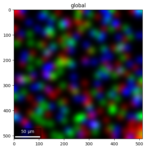
The default box is white, so on a dark image like blobs you either keep the default (dark bar on a white box) or, if you switch to color="white", pair it with a dark box (box_color/box_alpha) or frameon=False — otherwise the white bar lands on the white box and disappears.

sdata.pl.render_images("blobs_image").pl.show(
    scalebar_dx=PX_SIZE_UM,
    scalebar_units="um",
    scalebar_params={
        "location": "lower left",
        "color": "white",
        "box_color": "black",
        "box_alpha": 0.4,
        "length_fraction": 0.25,
        "scale_loc": "top",
    },
)

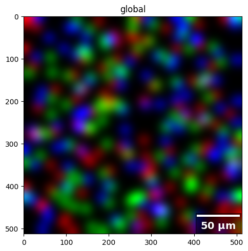
Font styling goes through font_properties, a matplotlib font dict:

sdata.pl.render_images("blobs_image").pl.show(
    scalebar_dx=PX_SIZE_UM,
    scalebar_units="um",
    scalebar_params={
        "location": "lower right",
        "color": "white",
        "box_color": "black",
        "box_alpha": 0.5,
        "font_properties": {"size": 14, "weight": "bold"},
    },
)

4. Pinning an exact bar length

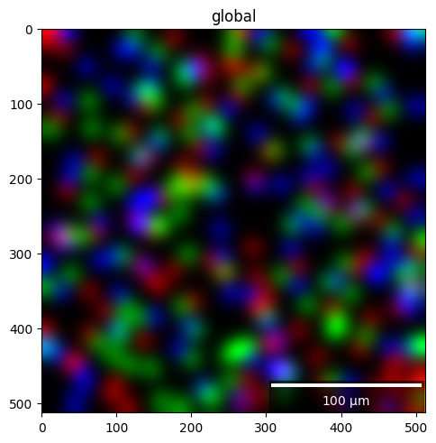
By default the bar snaps to a round length near length_fraction. To force an exact length — e.g. a 100 µm bar for a figure panel — set fixed_value (and fixed_units):

sdata.pl.render_images("blobs_image").pl.show(
    scalebar_dx=PX_SIZE_UM,
    scalebar_units="um",
    scalebar_params={
        "location": "lower right",
        "color": "white",
        "box_color": "black",
        "box_alpha": 0.5,
        "fixed_value": 100,
        "fixed_units": "um",
    },
)

5. Everything else, and on real data

Because scalebar_params is forwarded to matplotlib-scalebar, anything that library supports (rotation, width_fraction, custom formatters, …) works too — see the matplotlib-scalebar documentation for the full list.

For a scalebar on a real dataset with a genuine micron-per-pixel value, see the Visium mouse brain example, which finishes with a publication-style figure.

For reproducibility

# ruff: noqa: F401, F811, I001, E402
# fmt: off
import spatialdata_plot

%load_ext watermark
# fmt: on
%watermark -v -m -p spatialdata,spatialdata_plot,matplotlib,matplotlib_scalebar