Analysis of 3k T cells from cancer
In this tutorial, we re-analyze single-cell TCR/RNA-seq data from Wu et al. ([WMdA+20]) generated on the 10x Genomics platform. The original dataset consists of >140k T cells from 14 treatment-naive patients across four different types of cancer. For this tutorial, to speed up computations, we use a downsampled version of 3k cells.
[1]:
# This cell is for development only. Don't copy this to your notebook.
%load_ext autoreload
%autoreload 2
[2]:
import numpy as np
import pandas as pd
import scanpy as sc
import scirpy as ir
from matplotlib import pyplot as plt, cm as mpl_cm
from cycler import cycler

sc.set_figure_params(figsize=(4, 4))
sc.settings.verbosity = 2  # verbosity: errors (0), warnings (1), info (2), hints (3)
/opt/hostedtoolcache/Python/3.8.12/x64/lib/python3.8/site-packages/traitlets/traitlets.py:3044: FutureWarning: --rc={'figure.dpi': 96} for dict-traits is deprecated in traitlets 5.0. You can pass --rc <key=value> ... multiple times to add items to a dict.
  warn(
[3]:
sc.logging.print_header()
scanpy==1.8.1 anndata==0.7.6 umap==0.5.1 numpy==1.20.3 scipy==1.7.1 pandas==1.3.3 scikit-learn==0.24.2 statsmodels==0.13.0rc0 python-igraph==0.9.6 pynndescent==0.5.4
The dataset ships with the scirpy package. We can conveniently load it from the datasets module:
[4]:
adata = ir.datasets.wu2020_3k()
try downloading from url
https://github.com/icbi-lab/scirpy/releases/download/d0.1.0/wu2020_3k.h5ad
... this may take a while but only happens once
creating directory /home/runner/work/scirpy/scirpy/docs/tutorials/data/ for saving data
100%|██████████| 16.0M/16.0M [00:00<00:00, 124MB/s]
Note
adata is a regular AnnData object with additional, Immune Receptor (IR)-specific columns in obs that are named according to the AIRR Rearrangement Schema. For more information, check the page about
Scirpy’s data structure, and
Scirpy’s working model of immune receptors.
Warning
scirpy’s data structure has updated in v0.7.0 to be fully AIRR-compliant.
AnnData objects created with older versions of scirpy can be upgraded with scirpy.io.upgrade_schema() to be compatible with the latest version of scirpy.
[5]:
adata.shape
[5]:
(3000, 30727)
[6]:
adata.obs
[6]:
| cluster_orig | patient | sample | source | clonotype_orig | multi_chain | IR_VJ_1_locus | IR_VJ_2_locus | IR_VDJ_1_locus | IR_VDJ_2_locus | ... | IR_VJ_2_c_call | IR_VDJ_1_c_call | IR_VDJ_2_c_call | IR_VJ_1_junction | IR_VJ_2_junction | IR_VDJ_1_junction | IR_VDJ_2_junction | has_ir | batch | extra_chains | |
|---|---|---|---|---|---|---|---|---|---|---|---|---|---|---|---|---|---|---|---|---|---|
| LN1_GTAGGCCAGCGTAGTG-1-19 | 4.4-FOS | Lung1 | LN1 | NAT | lung1.tn.C223 | False | nan | nan | TRB | TRB | ... | nan | TRBC2 | TRBC2 | None | None | TGTGCCAGCAGCTTAATGCGGCTAGCGGGAGATACGCAGTATTTT | TGTGCAAGTCGCTTAGCGGTTTTATCGACTAGCGGGAGTGTCGGAG... | True | 19 | NaN |
| RN2_AGAGCGACAGATTGCT-1-27 | 4.4-FOS | Renal2 | RN2 | NAT | renal2.tnb.C1362 | False | TRA | nan | TRB | nan | ... | nan | TRBC1 | nan | TGTGCTGTGAGGGGGAATAACAATGCCAGACTCATGTTT | None | TGTGCCAGCAGCTTTGGAACGGTGGCTGAAGCTTTCTTT | None | True | 27 | NaN |
| LN1_GTCATTTCAATGAAAC-1-19 | 8.2-Tem | Lung1 | LN1 | NAT | lung1.tn.C25 | False | TRA | nan | TRB | nan | ... | nan | TRBC1 | nan | TGTGCTGTGAGGTTGGGTAACCAGTTCTATTTT | None | TGCAGTGCTAGAGATGGAGGGGGGGGGAACACTGAAGCTTTCTTT | None | True | 19 | NaN |
| LN2_GACACGCAGGTAGCTG-2-2 | 8.6-KLRB1 | Lung2 | LN2 | NAT | lung2.tn.C2452 | False | nan | nan | TRB | nan | ... | nan | TRBC2 | nan | None | None | TGTGCCAGCAGCCAAGGTCAGGGACAGGATTTTAACTACGAGCAGT... | None | True | 2 | NaN |
| LN2_GCACTCTCAGGGATTG-2-2 | 4.4-FOS | Lung2 | LN2 | NAT | lung2.tn.C5631 | False | TRA | nan | TRB | nan | ... | nan | TRBC1 | nan | TGTGCAGCAAGCGACCCCACGGTCGAGGCAGGAACTGCTCTGATCTTT | None | TGTGCCAGCAGCTTGACCGTTAACACTGAAGCTTTCTTT | None | True | 2 | NaN |
| ... | ... | ... | ... | ... | ... | ... | ... | ... | ... | ... | ... | ... | ... | ... | ... | ... | ... | ... | ... | ... | ... |
| RT3_GCAGTTAGTATGAAAC-1-6 | 4.2-RPL32 | Renal3 | RT3 | Tumor | renal3.tnb.C176 | False | TRA | nan | TRB | nan | ... | nan | TRBC2 | nan | TGTGCTGCGATGGATAGCAACTATCAGTTAATCTGG | None | TGTGCCACCAAGGACAGGGAAGACACCGGGGAGCTGTTTTTT | None | True | 6 | NaN |
| LT1_GACGTGCTCTCAAGTG-1-24 | 8.2-Tem | Lung1 | LT1 | Tumor | lung1.tn.C151 | False | TRA | nan | nan | nan | ... | nan | nan | nan | TGTGCTTATAGGAGTTCCCTTGGTGGTGCTACAAACAAGCTCATCTTT | None | None | None | True | 24 | NaN |
| ET3_GCTGGGTAGACCTTTG-1-3 | 3.1-MT | Endo3 | ET3 | Tumor | endo3.tn.C76 | False | nan | nan | TRB | nan | ... | nan | TRBC2 | nan | None | None | TGTGCCAGCAGCCGGACAGGGGGGGATTCCGGGGAGCTGTTTTTT | None | True | 3 | NaN |
| RT1_TAAGAGATCCTTAATC-1-8 | 4.5-IL6ST | Renal1 | RT1 | Tumor | renal1.tnb.C83 | False | TRA | nan | TRB | nan | ... | nan | TRBC2 | nan | TGTGCAATGAGCGAGATTTCTGGTGGCTACAATAAGCTGATTTTT | None | TGTGCCTGGAGTGACAGGTCAGACGAGCAGTACTTC | None | True | 8 | NaN |
| LN2_TCTGAGAAGGACACCA-2-2 | 4.6b-Treg | Lung2 | LN2 | NAT | lung2.tn.C6211 | False | TRA | nan | TRB | nan | ... | nan | TRBC2 | nan | TGTGCTACGGAGGAATATGGAAACAAGCTGGTCTTT | None | TGTGCCAGCAGCTTTCTACCTTTGGGAGATACGCAGTATTTT | None | True | 2 | NaN |
3000 rows × 45 columns
Note
Importing data
scirpy natively supports reading IR data from Cellranger (10x), TraCeR (Smart-seq2) or the AIRR rearrangement schema and provides helper functions to import other data types. We provide a dedicated tutorial on data loading with more details.
This particular dataset has been imported using scirpy.io.read_10x_vdj() and merged
with transcriptomics data using scirpy.pp.merge_with_ir(). The exact procedure
is described in scirpy.datasets.wu2020().
Preprocess Transcriptomics data
Transcriptomics data needs to be filtered and preprocessed as with any other single-cell dataset. We recommend following the scanpy tutorial and the best practice paper by Luecken et al.
[7]:
sc.pp.filter_genes(adata, min_cells=10)
sc.pp.filter_cells(adata, min_genes=100)
filtered out 18877 genes that are detected in less than 10 cells
[8]:
sc.pp.normalize_per_cell(adata, counts_per_cell_after=1000)
sc.pp.log1p(adata)
sc.pp.highly_variable_genes(adata, flavor="cell_ranger", n_top_genes=5000)
sc.tl.pca(adata)
sc.pp.neighbors(adata)
normalizing by total count per cell
    finished (0:00:00): normalized adata.X and added    'n_counts', counts per cell before normalization (adata.obs)
If you pass `n_top_genes`, all cutoffs are ignored.
extracting highly variable genes
    finished (0:00:00)
computing PCA
    on highly variable genes
    with n_comps=50
    finished (0:00:00)
computing neighbors
    using 'X_pca' with n_pcs = 50
    finished (0:00:02)
For the Wu2020 dataset, the authors already provide clusters and UMAP coordinates. Instead of performing clustering and cluster annotation ourselves, we will just use the provided data. The clustering and annotation methodology is described in their paper.
[9]:
adata.obsm["X_umap"] = adata.obsm["X_umap_orig"]
[10]:
mapping = {
    "nan": "other",
    "3.1-MT": "other",
    "4.1-Trm": "CD4_Trm",
    "4.2-RPL32": "CD4_RPL32",
    "4.3-TCF7": "CD4_TCF7",
    "4.4-FOS": "CD4_FOSS",
    "4.5-IL6ST": "CD4_IL6ST",
    "4.6a-Treg": "CD4_Treg",
    "4.6b-Treg": "CD4_Treg",
    "8.1-Teff": "CD8_Teff",
    "8.2-Tem": "CD8_Tem",
    "8.3a-Trm": "CD8_Trm",
    "8.3b-Trm": "CD8_Trm",
    "8.3c-Trm": "CD8_Trm",
    "8.4-Chrom": "other",
    "8.5-Mitosis": "other",
    "8.6-KLRB1": "other",
}
adata.obs["cluster"] = [mapping[x] for x in adata.obs["cluster_orig"]]
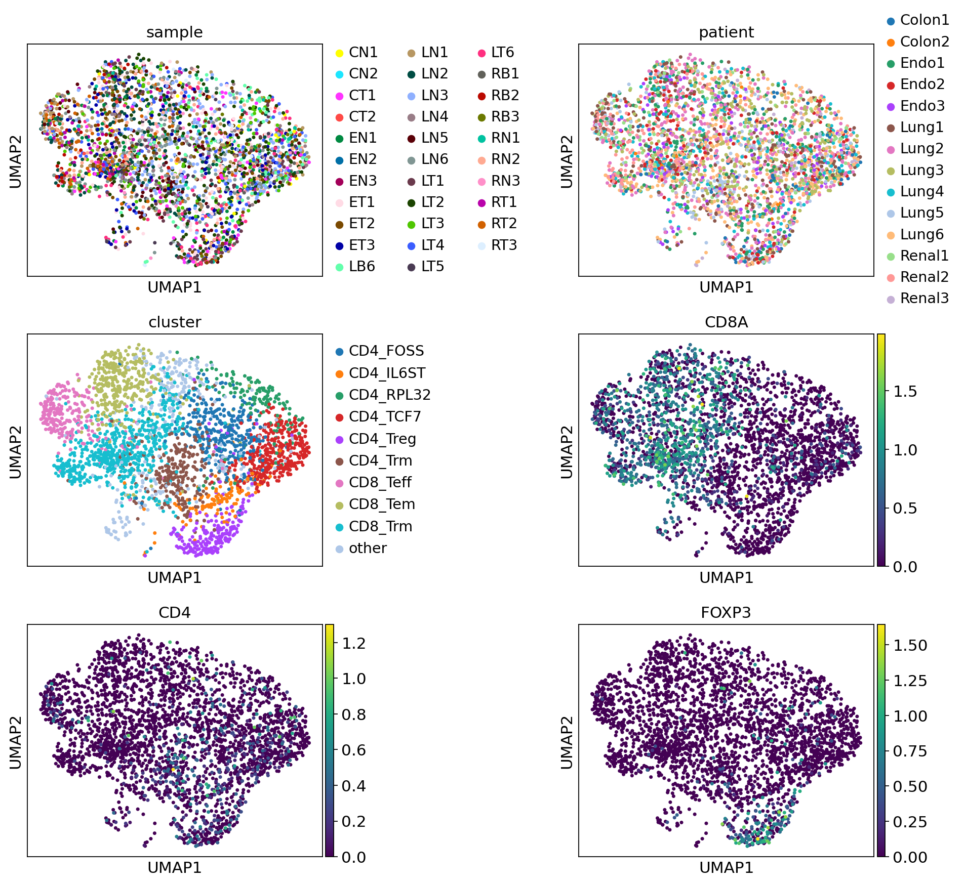
Let’s inspect the UMAP plots. The first three panels show the UMAP plot colored by sample, patient and cluster. We don’t observe any clustering of samples or patients that could hint at batch effects.
The last three panels show the UMAP colored by the T cell markers CD8, CD4, and FOXP3. We can confirm that the markers correspond to their respective cluster labels.
[11]:
sc.pl.umap(
    adata,
    color=["sample", "patient", "cluster", "CD8A", "CD4", "FOXP3"],
    ncols=2,
    wspace=0.7,
)
/opt/hostedtoolcache/Python/3.8.12/x64/lib/python3.8/site-packages/anndata/_core/anndata.py:1220: FutureWarning: The `inplace` parameter in pandas.Categorical.reorder_categories is deprecated and will be removed in a future version. Removing unused categories will always return a new Categorical object.
  c.reorder_categories(natsorted(c.categories), inplace=True)
... storing 'cluster' as categorical
TCR Quality Control
While most of T cell receptors have exactly one pair of α and β chains, up to one third of T cells can have dual TCRs, i.e. two pairs of receptors originating from different alleles ([SB19]).
Using the scirpy.tl.chain_qc() function, we can add a summary
about the Immune cell-receptor compositions to adata.obs. We can visualize it using scirpy.pl.group_abundance().
Note
chain pairing
Orphan chain refers to cells that have either a single alpha or beta receptor chain.
Extra chain refers to cells that have a full alpha/beta receptor pair, and an additional chain.
Multichain refers to cells with more than two receptor pairs detected. These cells are likely doublets.
Note
receptor type and receptor subtype
receptor_type refers to a coarse classification into BCR and TCR. Cells with both BCR and TCR chains are labelled as ambiguous.
receptor_subtype refers to a more specific classification into α/β, ɣ/δ, IG-λ, and IG-κ chain configurations.
For more details, see scirpy.tl.chain_qc().
[12]:
ir.tl.chain_qc(adata)
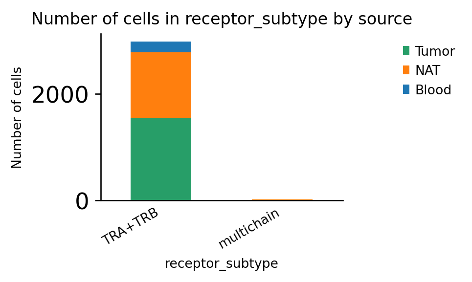
As expected, the dataset contains only α/β T-cell receptors:
[13]:
ax = ir.pl.group_abundance(adata, groupby="receptor_subtype", target_col="source")
/opt/hostedtoolcache/Python/3.8.12/x64/lib/python3.8/site-packages/anndata/_core/anndata.py:1220: FutureWarning: The `inplace` parameter in pandas.Categorical.reorder_categories is deprecated and will be removed in a future version. Removing unused categories will always return a new Categorical object.
  c.reorder_categories(natsorted(c.categories), inplace=True)
... storing 'receptor_type' as categorical
/opt/hostedtoolcache/Python/3.8.12/x64/lib/python3.8/site-packages/anndata/_core/anndata.py:1220: FutureWarning: The `inplace` parameter in pandas.Categorical.reorder_categories is deprecated and will be removed in a future version. Removing unused categories will always return a new Categorical object.
  c.reorder_categories(natsorted(c.categories), inplace=True)
... storing 'receptor_subtype' as categorical
/opt/hostedtoolcache/Python/3.8.12/x64/lib/python3.8/site-packages/anndata/_core/anndata.py:1220: FutureWarning: The `inplace` parameter in pandas.Categorical.reorder_categories is deprecated and will be removed in a future version. Removing unused categories will always return a new Categorical object.
  c.reorder_categories(natsorted(c.categories), inplace=True)
... storing 'chain_pairing' as categorical
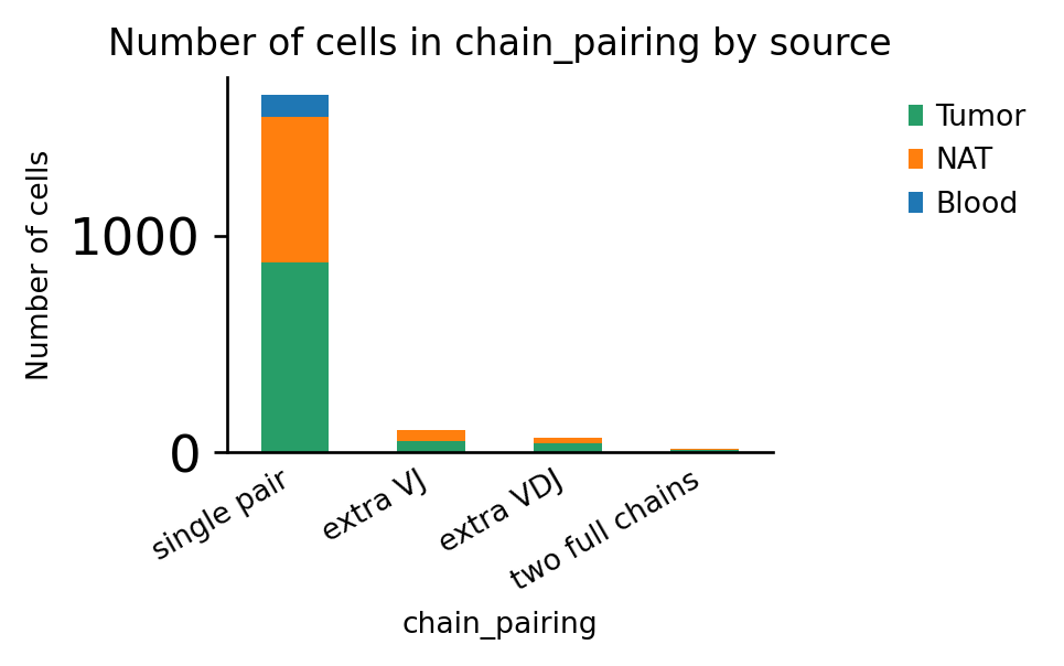
[14]:
ax = ir.pl.group_abundance(adata, groupby="chain_pairing", target_col="source")
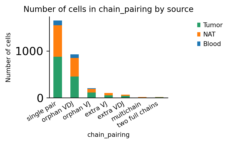
Indeed, in this dataset, ~6% of cells have more than one pair of productive T-cell receptors:
[15]:
print(
    "Fraction of cells with more than one pair of TCRs: {:.2f}".format(
        np.sum(
            adata.obs["chain_pairing"].isin(
                ["extra VJ", "extra VDJ", "two full chains"]
            )
        )
        / adata.n_obs
    )
)
Fraction of cells with more than one pair of TCRs: 0.06
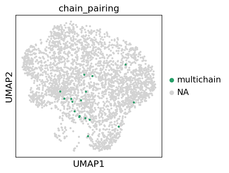
Next, we visualize the Multichain-cells on the UMAP plot and exclude them from downstream analysis:
[16]:
sc.pl.umap(adata, color="chain_pairing", groups="multichain")
[17]:
adata = adata[adata.obs["chain_pairing"] != "multichain", :].copy()
Similarly, we can use the chain_pairing information to exclude all cells that don’t have at least one full pair of receptor sequences:
[18]:
adata = adata[~adata.obs["chain_pairing"].isin(["orphan VDJ", "orphan VJ"]), :].copy()
Finally, we re-create the chain-pairing plot to ensure that the filtering worked as expected:
[19]:
ax = ir.pl.group_abundance(adata, groupby="chain_pairing", target_col="source")
Define clonotypes and clonotype clusters
Warning
The way scirpy computes clonotypes and clonotype clusters has been changed in v0.7.0.
Code written based on scirpy versions prior to v0.7.0 needs to be updated. Please read the release notes and follow the description in this section.
In this section, we will define and visualize clonotypes and clonotype clusters.
Scirpy implements a network-based approach for clonotype definition. The steps to create and visualize the clonotype-network are analogous to the construction of a neighborhood graph from transcriptomics data with scanpy.
scirpy function |
objective |
|---|---|
Compute sequence-based distance matrices for all VJ and VDJ sequences. |
|
Define clonotypes by nucleotide sequence identity. |
|
Cluster cells by the similarity of their CDR3-sequences. |
|
Compute layout of the clonotype network. |
|
Plot clonotype network colored by different parameters. |
Compute CDR3 neighborhood graph and define clonotypes
scirpy.pp.ir_dist() computes distances between CDR3 nucleotide (nt) or amino acid (aa) sequences, either based on sequence identity or similarity. It creates two distance matrices: one for all unique VJ sequences and one for all unique VDJ sequences. The distance matrices are added to adata.uns.
The function scirpy.tl.define_clonotypes() matches cells based on the distances of their
VJ and VDJ CDR3-sequences and value of the function parameters dual_ir and receptor_arms. Finally, it
detects connected modules in the graph and annotates them as clonotypes. This will add a clone_id and
clone_id_size column to adata.obs.
The dual_ir parameter defines how scirpy handles cells with more than one pair of receptors. The default value is any which implies that cells with any of their primary or secondary receptor chain matching will be considered to be of the same clonotype.
Here, we define clonotypes based on nt-sequence identity. In a later step, we will define clonotype clusters based on amino-acid similarity.
[20]:
# using default parameters, `ir_dist` will compute nucleotide sequence identity
ir.pp.ir_dist(adata)
ir.tl.define_clonotypes(adata, receptor_arms="all", dual_ir="primary_only")
Computing sequence x sequence distance matrix for VJ sequences.
Computing sequence x sequence distance matrix for VDJ sequences.
Initializing lookup tables.
Computing clonotype x clonotype distances.
100%|██████████| 1526/1526 [00:02<00:00, 590.01it/s]
Stored clonal assignments in `adata.obs["clone_id"]`.
To visualize the network we first call scirpy.tl.clonotype_network() to compute the layout.
We can then visualize it using scirpy.pl.clonotype_network(). We recommend setting the
min_cells parameter to >=2, to prevent the singleton clonotypes from cluttering the network.
[21]:
ir.tl.clonotype_network(adata, min_cells=2)
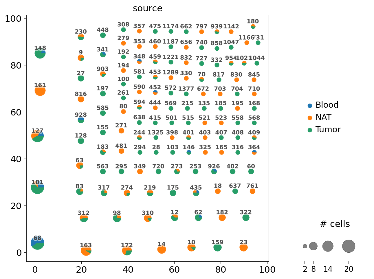
The resulting plot is a network, where each dot represents cells with identical receptor configurations. As we define clonotypes as cells with identical CDR3-sequences, each dot is also a clonotype. For each clonotype, the numeric clonotype id is shown in the graph. The size of each dot refers to the number of cells with the same receptor configurations. Categorical variables can be visualized as pie charts.
[22]:
ir.pl.clonotype_network(
    adata, color="source", base_size=20, label_fontsize=9, panel_size=(7, 7)
)
/opt/hostedtoolcache/Python/3.8.12/x64/lib/python3.8/site-packages/anndata/_core/anndata.py:1220: FutureWarning: The `inplace` parameter in pandas.Categorical.reorder_categories is deprecated and will be removed in a future version. Removing unused categories will always return a new Categorical object.
  c.reorder_categories(natsorted(c.categories), inplace=True)
... storing 'clone_id' as categorical
[22]:
<AxesSubplot:>
Re-compute CDR3 neighborhood graph and define clonotype clusters
We can now re-compute the clonotype network based on amino-acid sequence similarity and define clonotype clusters.
To this end, we need to change set metric=”alignment” and specify a cutoff parameter. The distance is based on the BLOSUM62 matrix. For instance, a distance of 10 is equivalent to 2 R`s mutating into `N. This appoach was initially proposed as TCRdist by Dash et al. ([DFGH+17]).
All cells with a distance between their CDR3 sequences lower than cutoff will be connected in the network.
[23]:
ir.pp.ir_dist(
    adata,
    metric="alignment",
    sequence="aa",
    cutoff=15,
)
Computing sequence x sequence distance matrix for VJ sequences.
100%|██████████| 496/496 [00:13<00:00, 35.60it/s]
Computing sequence x sequence distance matrix for VDJ sequences.
100%|██████████| 496/496 [00:13<00:00, 35.58it/s]
[24]:
ir.tl.define_clonotype_clusters(
    adata, sequence="aa", metric="alignment", receptor_arms="all", dual_ir="any"
)
Initializing lookup tables.
Computing clonotype x clonotype distances.
100%|██████████| 1549/1549 [00:07<00:00, 197.82it/s]
Stored clonal assignments in `adata.obs["cc_aa_alignment"]`.
[25]:
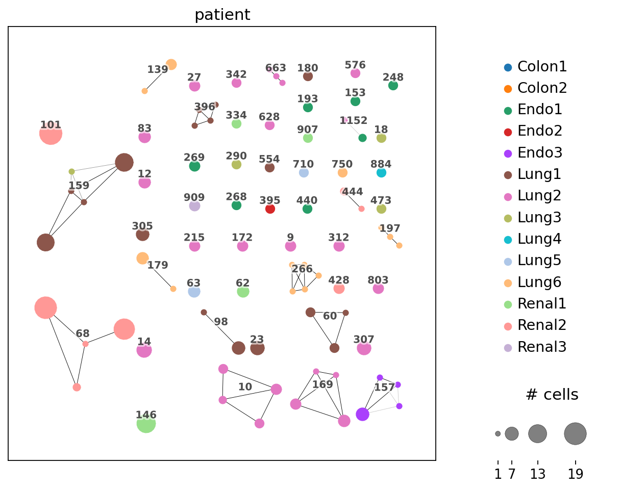
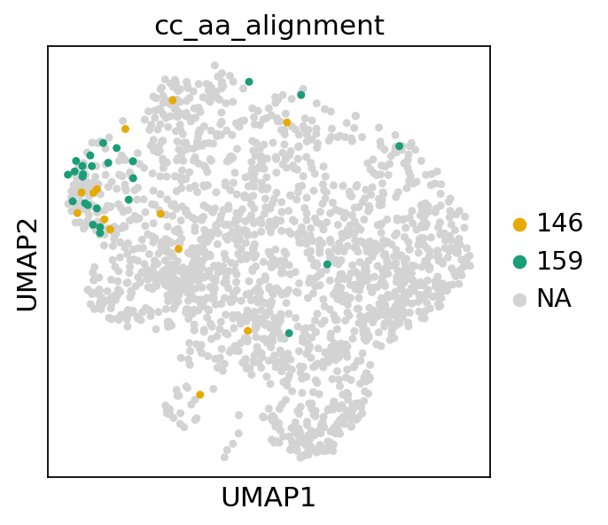
ir.tl.clonotype_network(adata, min_cells=3, sequence="aa", metric="alignment")
Compared to the previous plot, we observere several connected dots. Each fully connected subnetwork represents a “clonotype cluster”, each dot still represents cells with identical receptor configurations.
The dots are colored by patient. We observe, that for instance, clonotypes 101 and 68 (left top and bottom) are private, i.e. they contain cells from a single patient only. On the other hand, clonotype 159 (left middle) is public, i.e. it is shared across patients Lung1 and Lung3.
[26]:
ir.pl.clonotype_network(
    adata, color="patient", label_fontsize=9, panel_size=(7, 7), base_size=20
)
/opt/hostedtoolcache/Python/3.8.12/x64/lib/python3.8/site-packages/anndata/_core/anndata.py:1220: FutureWarning: The `inplace` parameter in pandas.Categorical.reorder_categories is deprecated and will be removed in a future version. Removing unused categories will always return a new Categorical object.
  c.reorder_categories(natsorted(c.categories), inplace=True)
... storing 'cc_aa_alignment' as categorical
[26]:
<AxesSubplot:>
We can now extract information (e.g. CDR3-sequences) from a specific clonotype cluster by subsetting AnnData. When extracting the CDR3 sequences of clonotype cluster 159, we retreive five different receptor configurations with different numbers of cells, corresponding to the five points in the graph.
[27]:
adata.obs.loc[adata.obs["cc_aa_alignment"] == "159", :].groupby(
    [
        "IR_VJ_1_junction_aa",
        "IR_VJ_2_junction_aa",
        "IR_VDJ_1_junction_aa",
        "IR_VDJ_2_junction_aa",
        "receptor_subtype",
    ],
    observed=True,
).size().reset_index(name="n_cells")
[27]:
| IR_VJ_1_junction_aa | IR_VJ_2_junction_aa | IR_VDJ_1_junction_aa | IR_VDJ_2_junction_aa | receptor_subtype | n_cells | |
|---|---|---|---|---|---|---|
| 0 | CAGKSGNTGKLIF | None | CASSYQGATEAFF | None | TRA+TRB | 12 |
| 1 | CAGKSGNTGKLIF | CATDPRRSTGNQFYF | CASSYQGATEAFF | None | TRA+TRB | 1 |
| 2 | CATDPRRSTGNQFYF | None | CASSYQGATEAFF | None | TRA+TRB | 11 |
| 3 | CATDPRRSTGNQFYF | CAGKSGNTGKLIF | CASSYQGATEAFF | None | TRA+TRB | 1 |
| 4 | CAGKAGNTGKLIF | None | CASSYQGSTEAFF | None | TRA+TRB | 1 |
Including the V-gene in clonotype definition
Using the paramter use_v_gene in define_clonotypes(), we can enforce
clonotypes (or clonotype clusters) to have the same V-gene, and, therefore, the same CDR1 and 2
regions. Let’s look for clonotype clusters with different V genes:
[28]:
ir.tl.define_clonotype_clusters(
    adata,
    sequence="aa",
    metric="alignment",
    receptor_arms="all",
    dual_ir="any",
    same_v_gene=True,
    key_added="cc_aa_alignment_same_v",
)
Initializing lookup tables.
Computing clonotype x clonotype distances.
100%|██████████| 1549/1549 [00:08<00:00, 180.84it/s]
Stored clonal assignments in `adata.obs["cc_aa_alignment_same_v"]`.
[29]:
# find clonotypes with more than one `clonotype_same_v`
ct_different_v = adata.obs.groupby("cc_aa_alignment").apply(
    lambda x: x["cc_aa_alignment_same_v"].nunique() > 1
)
ct_different_v = ct_different_v[ct_different_v].index.values.tolist()
ct_different_v
[29]:
['280', '765']
Here, we see that the clonotype clusters 280 and 765 get split into (280, 788) and (765, 1071), respectively, when the same_v_gene flag is set.
[30]:
adata.obs.loc[
    adata.obs["cc_aa_alignment"].isin(ct_different_v),
    [
        "cc_aa_alignment",
        "cc_aa_alignment_same_v",
        "IR_VJ_1_v_call",
        "IR_VDJ_1_v_call",
    ],
].sort_values("cc_aa_alignment").drop_duplicates().reset_index(drop=True)
[30]:
| cc_aa_alignment | cc_aa_alignment_same_v | IR_VJ_1_v_call | IR_VDJ_1_v_call | |
|---|---|---|---|---|
| 0 | 280 | 280 | TRAV8-6 | TRBV6-6 |
| 1 | 280 | 788 | TRAV8-3 | TRBV9 |
| 2 | 765 | 765 | TRAV21 | TRBV6-6 |
| 3 | 765 | 1071 | TRAV21 | TRBV6-5 |
Clonotype analysis
Clonal expansion
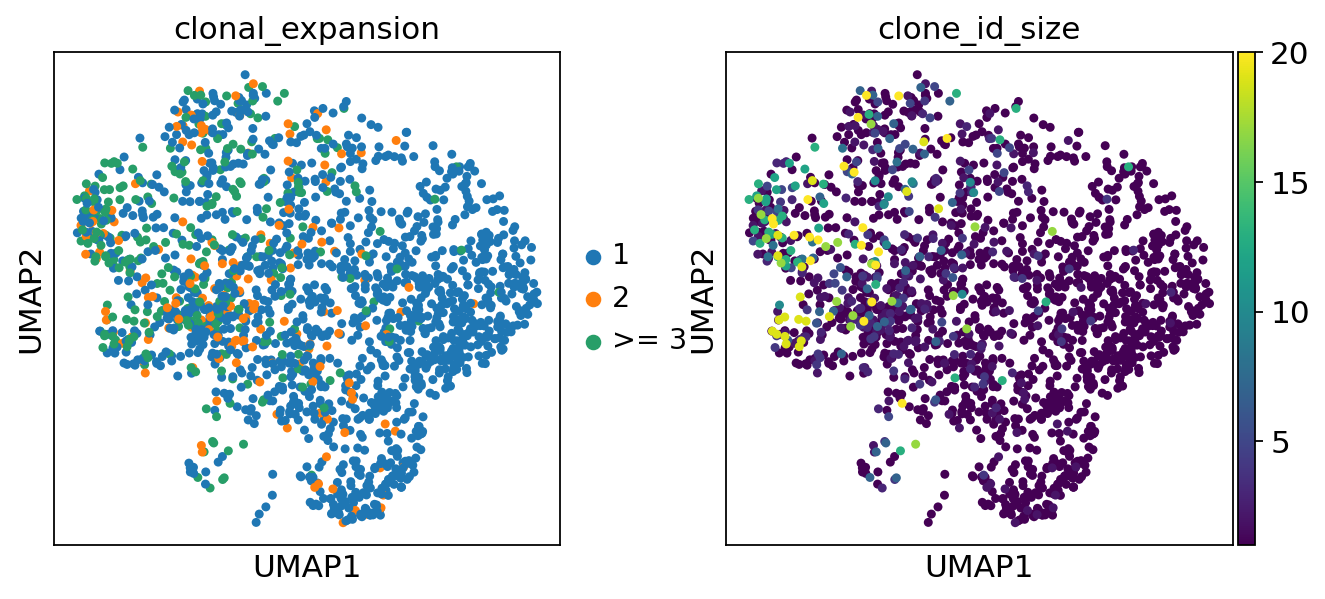
Let’s visualize the number of expanded clonotypes (i.e. clonotypes consisting
of more than one cell) by cell-type. The first option is to add a column with the scirpy.tl.clonal_expansion()
to adata.obs and overlay it on the UMAP plot.
[31]:
ir.tl.clonal_expansion(adata)
clonal_expansion refers to expansion categories, i.e singleton clonotypes, clonotypes with 2 cells and more than 2 cells. The clonotype_size refers to the absolute number of cells in a clonotype.
[32]:
sc.pl.umap(adata, color=["clonal_expansion", "clone_id_size"])
/opt/hostedtoolcache/Python/3.8.12/x64/lib/python3.8/site-packages/anndata/_core/anndata.py:1220: FutureWarning: The `inplace` parameter in pandas.Categorical.reorder_categories is deprecated and will be removed in a future version. Removing unused categories will always return a new Categorical object.
  c.reorder_categories(natsorted(c.categories), inplace=True)
... storing 'cc_aa_alignment_same_v' as categorical
/opt/hostedtoolcache/Python/3.8.12/x64/lib/python3.8/site-packages/anndata/_core/anndata.py:1220: FutureWarning: The `inplace` parameter in pandas.Categorical.reorder_categories is deprecated and will be removed in a future version. Removing unused categories will always return a new Categorical object.
  c.reorder_categories(natsorted(c.categories), inplace=True)
... storing 'clonal_expansion' as categorical
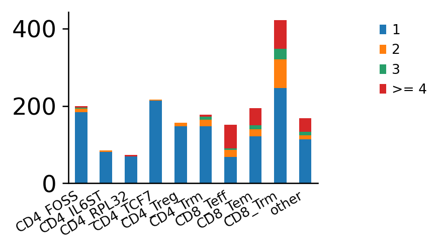
The second option is to show the number of cells belonging to an expanded clonotype per category
in a stacked bar plot, using the scirpy.pl.clonal_expansion() plotting function.
[33]:
ir.pl.clonal_expansion(adata, groupby="cluster", clip_at=4, normalize=False)
[33]:
<AxesSubplot:>
The same plot, normalized to cluster size. Clonal expansion is a sign of positive selection for a certain, reactive T-cell clone. It, therefore, makes sense that CD8+ effector T-cells have the largest fraction of expanded clonotypes.
[34]:
ir.pl.clonal_expansion(adata, "cluster")
[34]:
<AxesSubplot:>
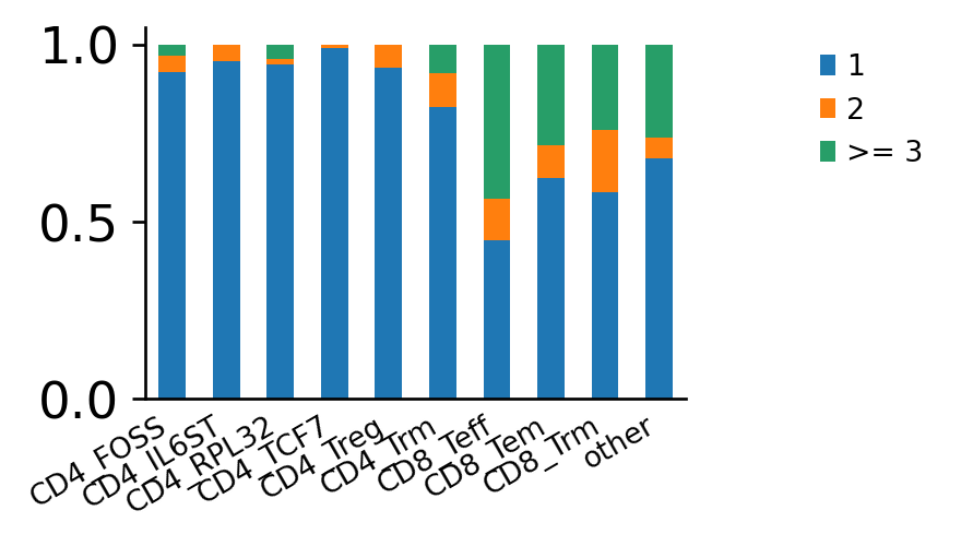
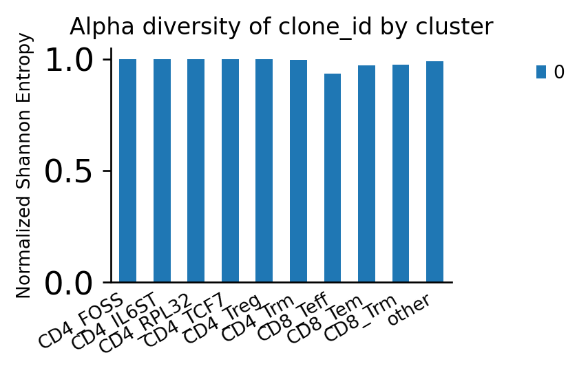
Expectedly, the CD8+ effector T cells have the largest fraction of expanded clonotypes.
Consistent with this observation, they have the lowest scirpy.pl.alpha_diversity() of clonotypes.
[35]:
ax = ir.pl.alpha_diversity(
    adata, metric="normalized_shannon_entropy", groupby="cluster"
)
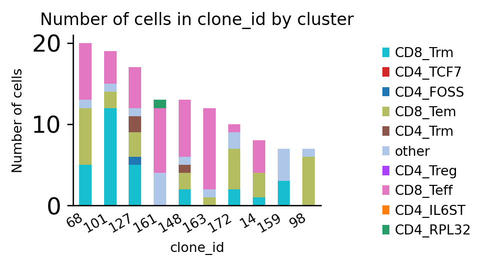
Clonotype abundance
The function scirpy.pl.group_abundance() allows us to create bar charts for
arbitrary categorial from obs. Here, we use it to show the distribution of the
ten largest clonotypes across the cell-type clusters.
[36]:
ir.pl.group_abundance(adata, groupby="clone_id", target_col="cluster", max_cols=10)
[36]:
<AxesSubplot:title={'center':'Number of cells in clone_id by cluster'}, xlabel='clone_id', ylabel='Number of cells'>
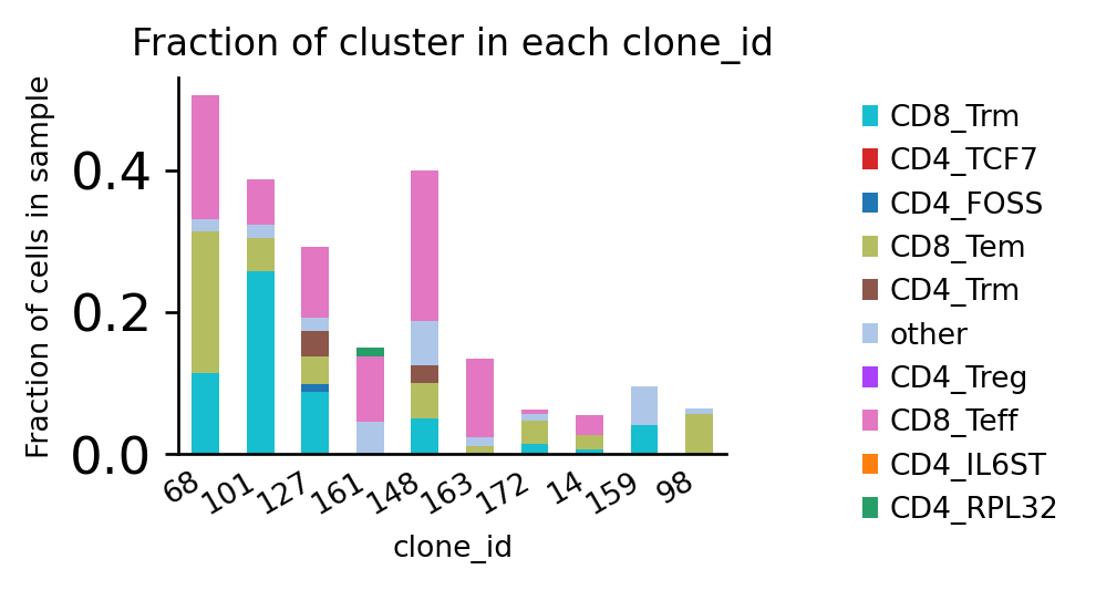
It might be beneficial to normalize the counts to the number of cells per sample to mitigate biases due to different sample sizes:
[37]:
ir.pl.group_abundance(
    adata, groupby="clone_id", target_col="cluster", max_cols=10, normalize="sample"
)
[37]:
<AxesSubplot:title={'center':'Fraction of cluster in each clone_id'}, xlabel='clone_id', ylabel='Fraction of cells in sample'>
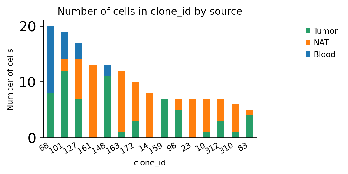
Coloring the bars by patient gives us information about public and private clonotypes: Some clonotypes are private, i.e. specific to a certain tissue, others are public, i.e. they are shared across different tissues.
[38]:
ax = ir.pl.group_abundance(
    adata, groupby="clone_id", target_col="source", max_cols=15, figsize=(5, 3)
)
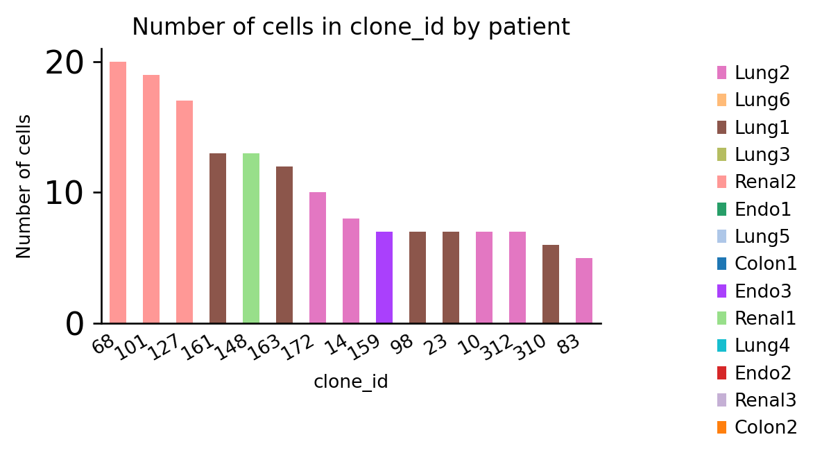
However, clonotypes that are shared between patients are rare:
[39]:
ax = ir.pl.group_abundance(
    adata, groupby="clone_id", target_col="patient", max_cols=15, figsize=(5, 3)
)
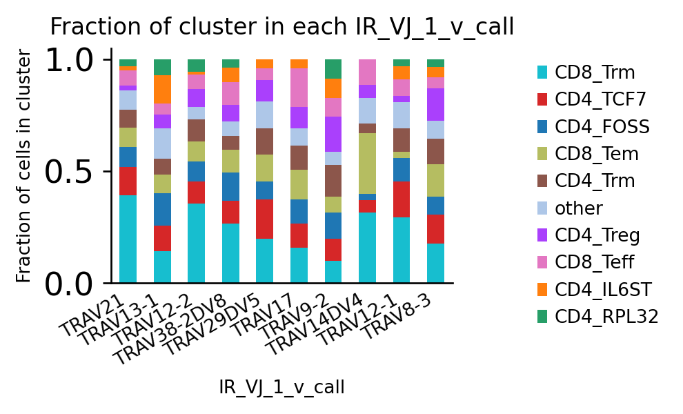
Gene usage
scirpy.tl.group_abundance() can also give us some information on VDJ usage.
We can choose any of the {TRA,TRB}_{1,2}_{v,d,j,c}_gene columns to make a stacked bar plot.
We use max_col to limit the plot to the 10 most abundant V-genes.
[40]:
ax = ir.pl.group_abundance(
    adata, groupby="IR_VJ_1_v_call", target_col="cluster", normalize=True, max_cols=10
)
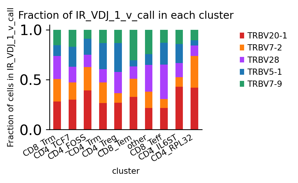
We can pre-select groups by filtering adata:
[41]:
ax = ir.pl.group_abundance(
    adata[
        adata.obs["IR_VDJ_1_v_call"].isin(
            ["TRBV20-1", "TRBV7-2", "TRBV28", "TRBV5-1", "TRBV7-9"]
        ),
        :,
    ],
    groupby="cluster",
    target_col="IR_VDJ_1_v_call",
    normalize=True,
)
Trying to set attribute `.uns` of view, copying.
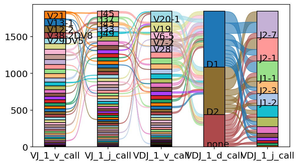
The exact combinations of VDJ genes can be visualized as a Sankey-plot using scirpy.pl.vdj_usage().
[42]:
ax = ir.pl.vdj_usage(adata, full_combination=False, max_segments=None, max_ribbons=30)
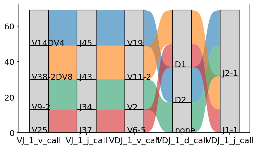
We can also use this plot to investigate the exact VDJ composition of one (or several) clonotypes:
[43]:
ir.pl.vdj_usage(
    adata[adata.obs["clone_id"].isin(["68", "101", "127", "161"]), :],
    max_ribbons=None,
    max_segments=100,
)
[43]:
<AxesSubplot:>
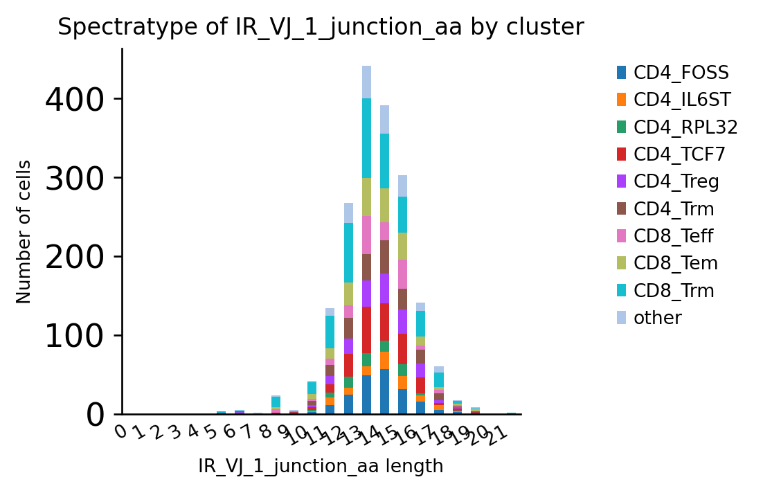
Spectratype plots
spectratype() plots give us information about the length distribution of CDR3 regions.
[44]:
ir.pl.spectratype(adata, color="cluster", viztype="bar", fig_kws={"dpi": 120})
[44]:
<AxesSubplot:title={'center':'Spectratype of IR_VJ_1_junction_aa by cluster'}, xlabel='IR_VJ_1_junction_aa length', ylabel='Number of cells'>
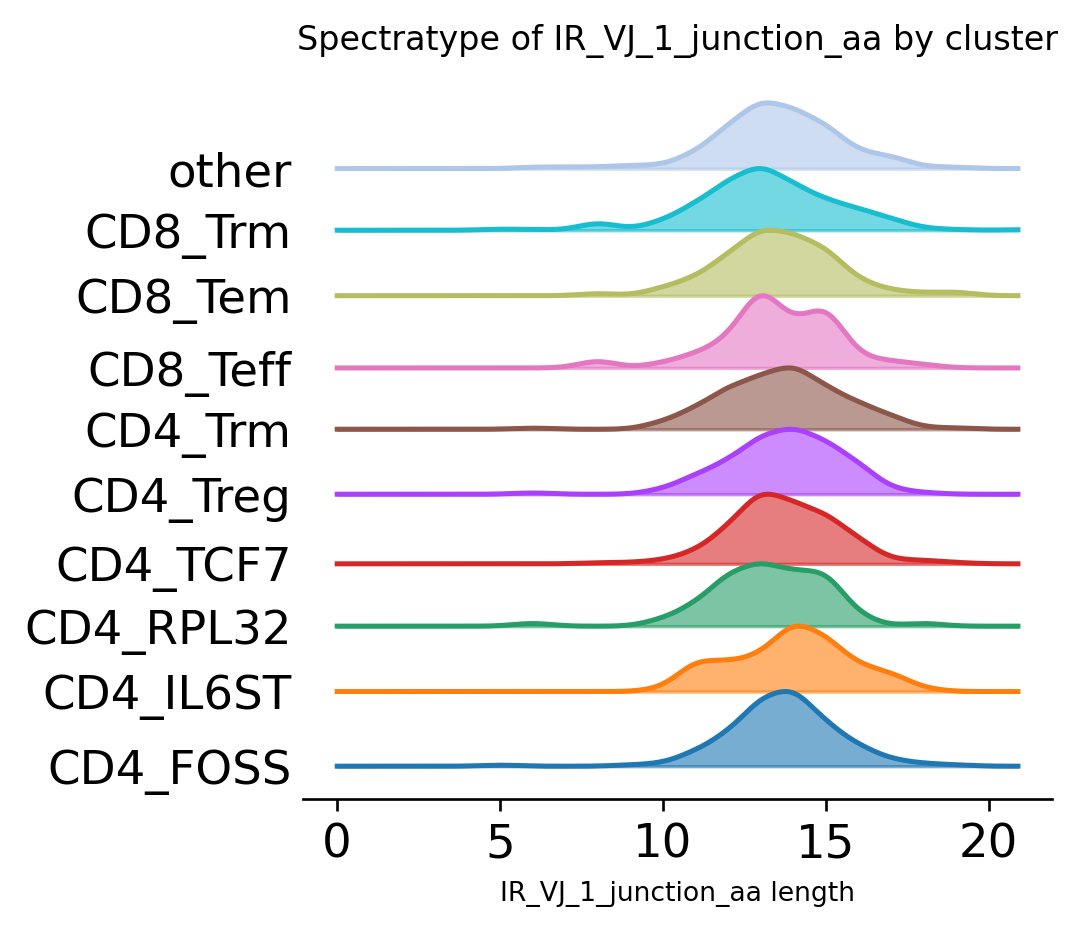
The same chart visualized as “ridge”-plot:
[45]:
ir.pl.spectratype(
    adata,
    color="cluster",
    viztype="curve",
    curve_layout="shifted",
    fig_kws={"dpi": 120},
    kde_kws={"kde_norm": False},
)
/opt/hostedtoolcache/Python/3.8.12/x64/lib/python3.8/site-packages/scirpy/_plotting/base.py:262: UserWarning: FixedFormatter should only be used together with FixedLocator
  ax.set_yticklabels(order)
[45]:
<AxesSubplot:title={'center':'Spectratype of IR_VJ_1_junction_aa by cluster'}, xlabel='IR_VJ_1_junction_aa length'>
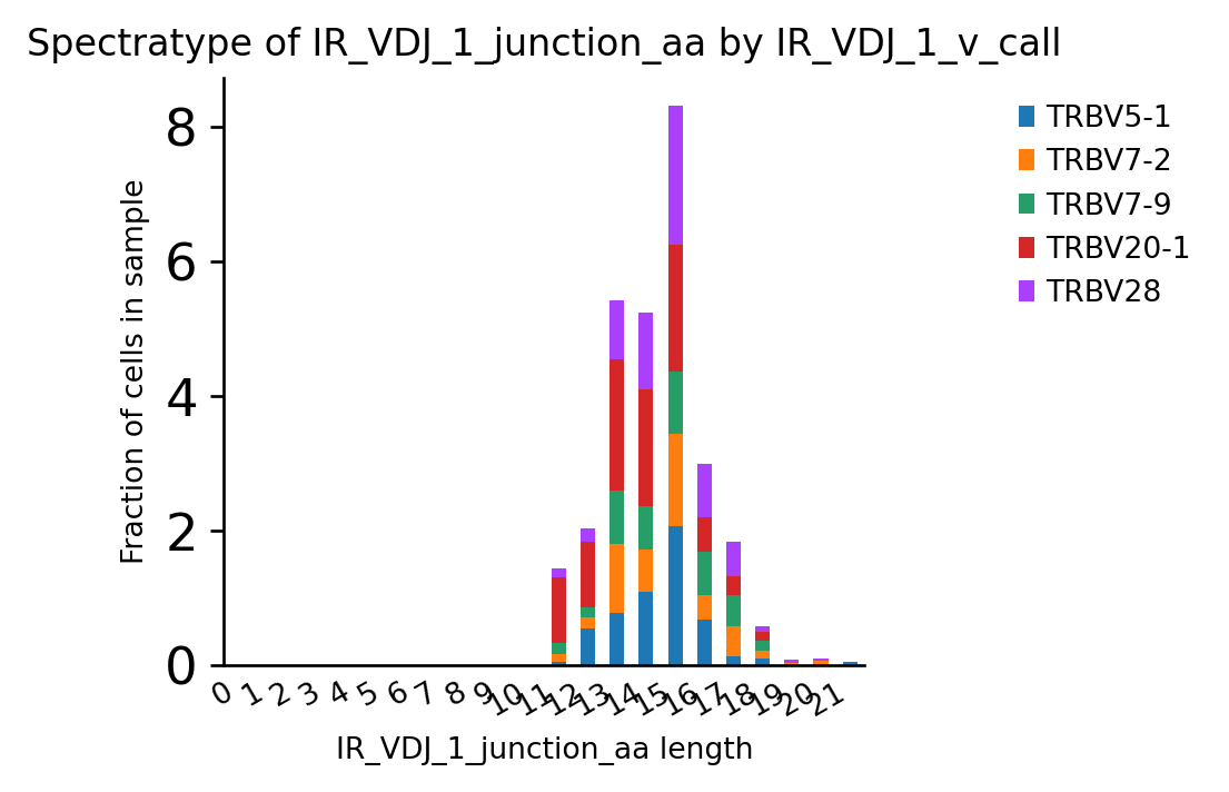
A spectratype-plot by gene usage. To pre-select specific genes, we can simply filter the adata object before plotting.
[46]:
ir.pl.spectratype(
    adata[
        adata.obs["IR_VDJ_1_v_call"].isin(
            ["TRBV20-1", "TRBV7-2", "TRBV28", "TRBV5-1", "TRBV7-9"]
        ),
        :,
    ],
    cdr3_col="IR_VDJ_1_junction_aa",
    color="IR_VDJ_1_v_call",
    normalize="sample",
    fig_kws={"dpi": 120},
)
Trying to set attribute `.uns` of view, copying.
[46]:
<AxesSubplot:title={'center':'Spectratype of IR_VDJ_1_junction_aa by IR_VDJ_1_v_call'}, xlabel='IR_VDJ_1_junction_aa length', ylabel='Fraction of cells in sample'>
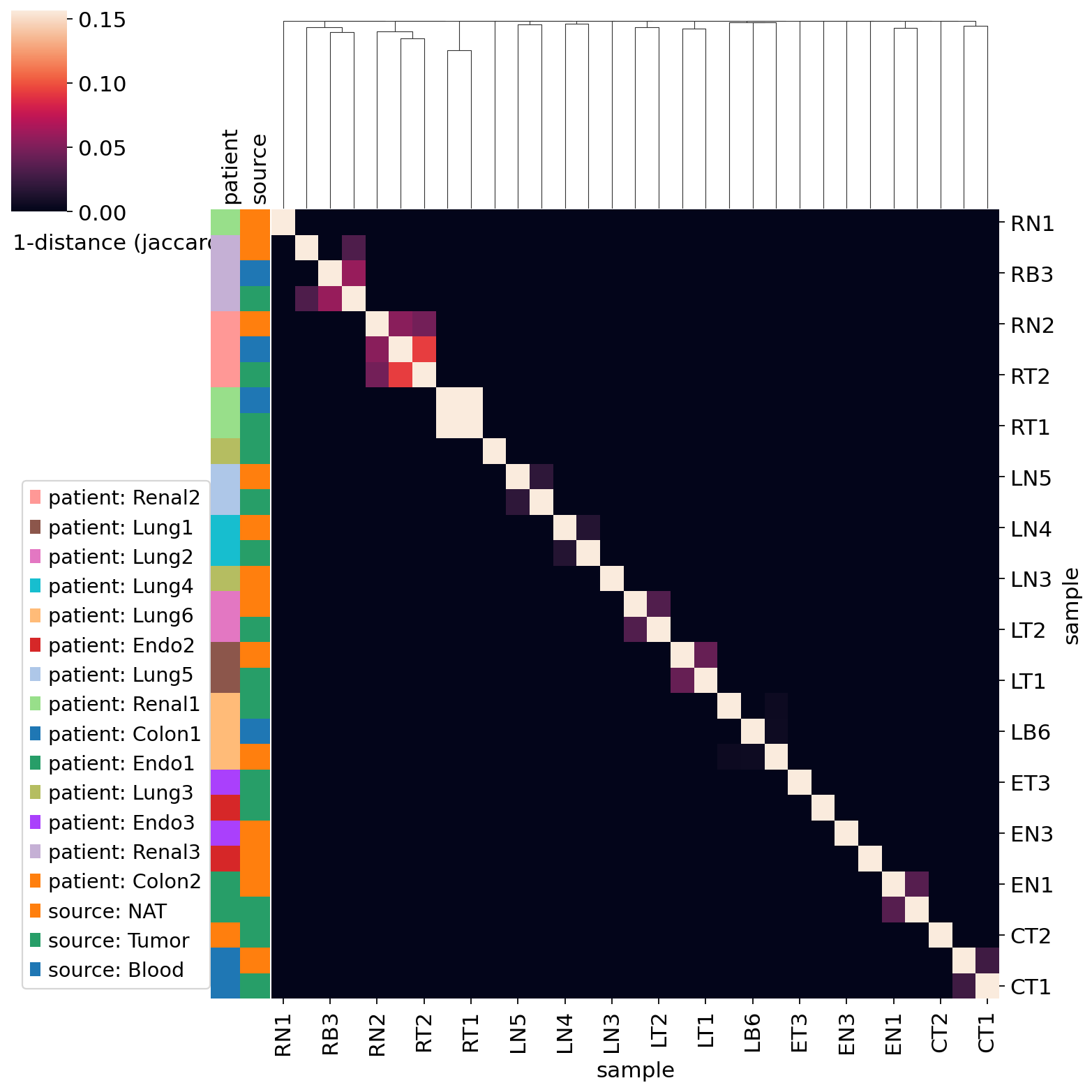
Comparing repertoires
Repertoire simlarity and overlaps
Overlaps in the adaptive immune receptor repertoire of samples or sample groups enables to pinpoint important clonotype groups, as well as to provide a measure of similarity between samples.
Running Scirpy’s repertoire_overlap() tool creates a matrix featuring the abundance of clonotypes in each sample. Additionally, it also computes a (Jaccard) distance matrix of samples as well as the linkage of hierarchical clustering.
[47]:
df, dst, lk = ir.tl.repertoire_overlap(adata, "sample", inplace=False)
df.head()
[47]:
| clone_id | 0 | 1 | 2 | 3 | 4 | 5 | 6 | 7 | 8 | 9 | ... | 1516 | 1517 | 1518 | 1519 | 1520 | 1521 | 1522 | 1523 | 1524 | 1525 |
|---|---|---|---|---|---|---|---|---|---|---|---|---|---|---|---|---|---|---|---|---|---|
| sample | |||||||||||||||||||||
| CN1 | 0.0 | 0.0 | 0.0 | 0.0 | 0.0 | 0.0 | 0.0 | 0.0 | 0.0 | 0.0 | ... | 0.0 | 0.0 | 0.0 | 0.0 | 0.0 | 0.0 | 0.0 | 0.0 | 0.0 | 0.0 |
| CT1 | 0.0 | 0.0 | 0.0 | 0.0 | 0.0 | 0.0 | 0.0 | 0.0 | 0.0 | 0.0 | ... | 0.0 | 0.0 | 0.0 | 0.0 | 1.0 | 0.0 | 0.0 | 0.0 | 0.0 | 0.0 |
| CT2 | 0.0 | 0.0 | 0.0 | 0.0 | 0.0 | 0.0 | 0.0 | 0.0 | 0.0 | 0.0 | ... | 0.0 | 0.0 | 0.0 | 0.0 | 0.0 | 0.0 | 0.0 | 0.0 | 0.0 | 0.0 |
| EN1 | 0.0 | 0.0 | 0.0 | 0.0 | 0.0 | 0.0 | 0.0 | 0.0 | 0.0 | 0.0 | ... | 0.0 | 0.0 | 0.0 | 0.0 | 0.0 | 0.0 | 0.0 | 0.0 | 0.0 | 0.0 |
| EN2 | 0.0 | 0.0 | 0.0 | 0.0 | 0.0 | 0.0 | 0.0 | 0.0 | 0.0 | 0.0 | ... | 0.0 | 0.0 | 0.0 | 0.0 | 0.0 | 0.0 | 0.0 | 0.0 | 0.0 | 0.0 |
5 rows × 1526 columns
The distance matrix can be shown as a heatmap, while samples are reordered based on hierarchical clustering.
[48]:
ir.pl.repertoire_overlap(adata, "sample", heatmap_cats=["patient", "source"])
[48]:
<seaborn.matrix.ClusterGrid at 0x7f94380b2250>
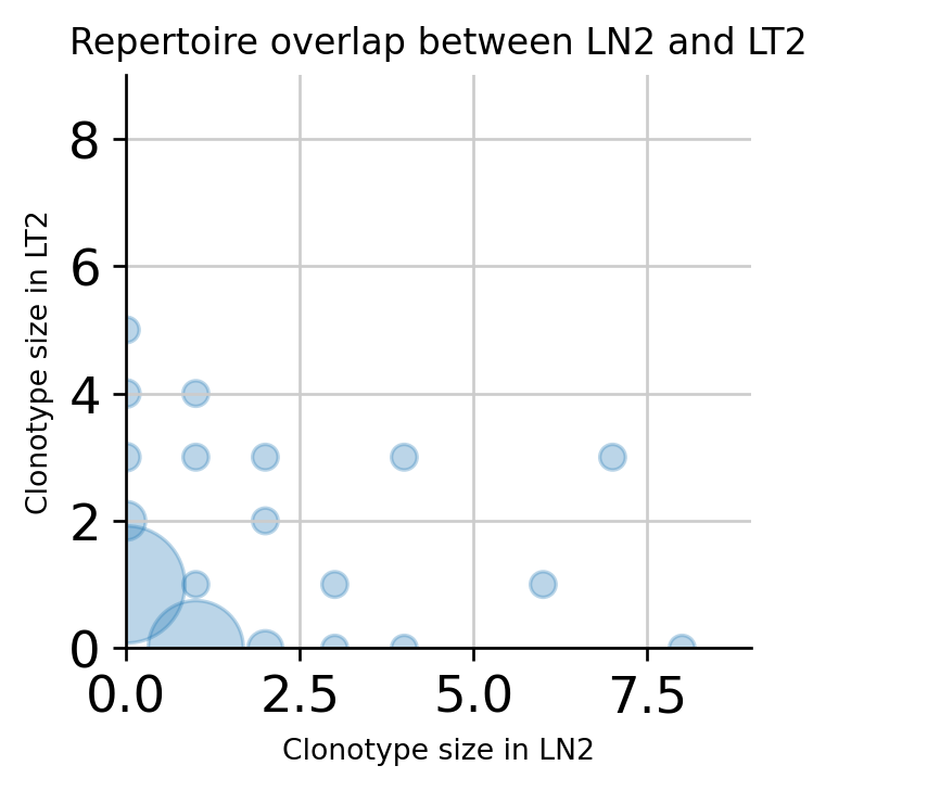
A specific pair of samples can be compared on a scatterplot, where dot size corresponds to the number of clonotypes at a given coordinate.
[49]:
ir.pl.repertoire_overlap(
    adata, "sample", pair_to_plot=["LN2", "LT2"], fig_kws={"dpi": 120}
)
No handles with labels found to put in legend.
[49]:
<AxesSubplot:title={'center':'Repertoire overlap between LN2 and LT2'}, xlabel='Clonotype size in LN2', ylabel='Clonotype size in LT2'>
Integrating gene expression data
Leveraging the opportunity offered by close integeration with scanpy, transcriptomics-based data can be utilized alongside immune receptor data.
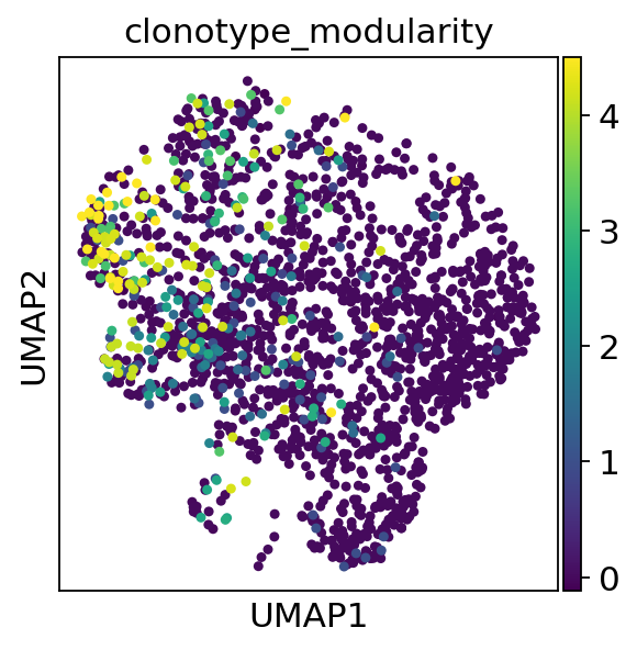
Clonotype modularity
Using the Clonotype modularity we can identify clonotypes consisting of cells that are transcriptionally more similar than expected by random.
The clonotype modularity score represents the log2 fold change of the number of edges in the cell-cell neighborhood graph compared to the random background model. Clonotypes (or clonotype clusters) with a high modularity score consist of cells that have a similar molecular phenotype.
[50]:
ir.tl.clonotype_modularity(adata, target_col="cc_aa_alignment")
Initalizing clonotype subgraphs...
100%|██████████| 1487/1487 [00:00<00:00, 6554.96it/s]
Computing background distributions...
100%|██████████| 1000/1000 [00:01<00:00, 766.86it/s]
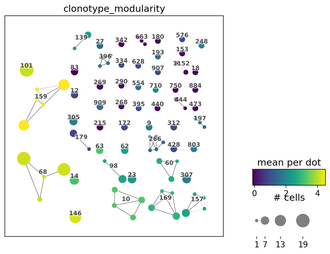
We can plot the clonotype modularity on top of a umap of clonotype network plot
[51]:
sc.pl.umap(adata, color="clonotype_modularity")
[52]:
ir.pl.clonotype_network(
    adata,
    color="clonotype_modularity",
    label_fontsize=9,
    panel_size=(6, 6),
    base_size=20,
)
[52]:
<AxesSubplot:>
We can also visualize the clonotype modularity together with the associated FDR as a sort of “one sided volcano plot”:
[53]:
ir.pl.clonotype_modularity(adata, base_size=20)
[53]:
<AxesSubplot:xlabel='modularity score', ylabel='-log10(FDR)'>
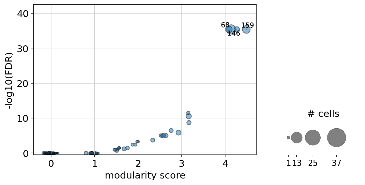
Let’s further inspect the two top scoring candidates. We can extract that information from adata.obs["clonotype_modularity"].
[54]:
clonotypes_top_modularity = list(
    adata.obs.set_index("cc_aa_alignment")["clonotype_modularity"]
    .sort_values(ascending=False)
    .index.unique().values[:2]
)
[55]:
sc.pl.umap(
    adata,
    color="cc_aa_alignment",
    groups=clonotypes_top_modularity,
    palette=cycler(color=mpl_cm.Dark2_r.colors),
)
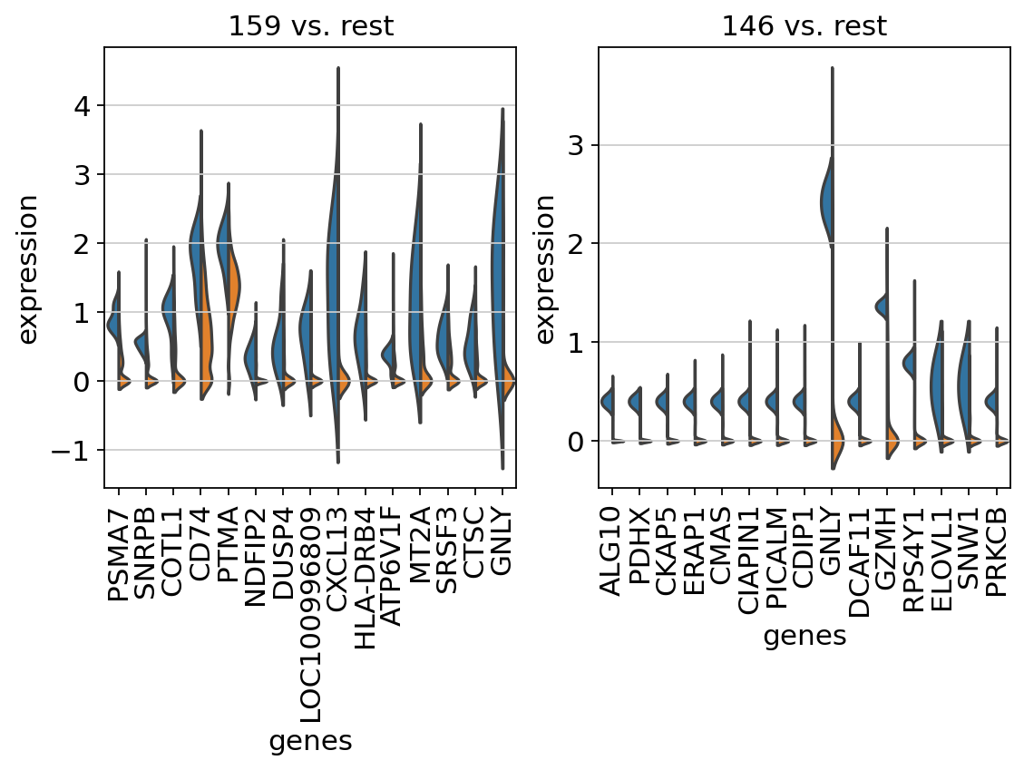
We observe that they are (mostly) restricted to a single cluster. By leveraging scanpy’s differential expression module, we can compare the gene expression of the cells in the two clonotypes to the rest.
[56]:
sc.tl.rank_genes_groups(
    adata, "clone_id", groups=clonotypes_top_modularity, reference="rest", method="wilcoxon"
)
fig, axs = plt.subplots(1, 2, figsize=(8, 4))
for ct, ax in zip(clonotypes_top_modularity, axs):
    sc.pl.rank_genes_groups_violin(adata, groups=[ct], n_genes=15, ax=ax, show=False, strip=False)
ranking genes
    finished (0:00:01)
Clonotype imbalance among cell clusters
Using cell type annotation inferred from gene expression clusters, for example, clonotypes belonging to CD8+ effector T-cells and CD8+ tissue-resident memory T cells, can be compared.
[57]:
freq, stat = ir.tl.clonotype_imbalance(
    adata,
    replicate_col="sample",
    groupby="cluster",
    case_label="CD8_Teff",
    control_label="CD8_Trm",
    inplace=False,
)
top_differential_clonotypes = stat["clone_id"].tolist()[:3]
WARNING: Clonotype imbalance calculation depends on repertoire overlap. We could not detect any previous runs of repertoire_overlap, so the tool is running now...
/opt/hostedtoolcache/Python/3.8.12/x64/lib/python3.8/site-packages/scirpy/io/_util.py:67: FutureWarning: clonotype_imbalance is a deprecated function and will be removed in a future version of scirpy. Consider using `tl.clonotype_modularity` instead. If `clonotype_modularity` does not cover your use-case, please create an issue on GitHub to let us know such that we can take it into account! (https://github.com/icbi-lab/scirpy/issues)
  return f(*args, **kwargs)
/opt/hostedtoolcache/Python/3.8.12/x64/lib/python3.8/site-packages/scirpy/_tools/_clonotype_imbalance.py:280: RuntimeWarning: divide by zero encountered in log2
  logfoldchange = np.log2(
/opt/hostedtoolcache/Python/3.8.12/x64/lib/python3.8/site-packages/scirpy/_tools/_clonotype_imbalance.py:281: RuntimeWarning: divide by zero encountered in double_scalars
  (case_mean_freq + global_minimum) / (control_mean_freq + global_minimum)
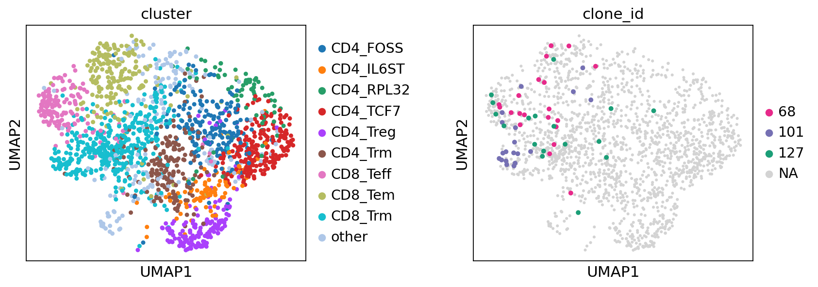
Showing top clonotypes on a UMAP clearly shows that clonotype 101 is featured by CD8+ tissue-resident memory T cells, while clonotype 68 by CD8+ effector and effector memory cells.
[58]:
fig, (ax1, ax2) = plt.subplots(1, 2, figsize=(12, 4), gridspec_kw={"wspace": 0.6})
sc.pl.umap(adata, color="cluster", ax=ax1, show=False)
sc.pl.umap(
    adata,
    color="clone_id",
    groups=top_differential_clonotypes,
    ax=ax2,
    # increase size of highlighted dots
    size=[
        80 if c in top_differential_clonotypes else 30 for c in adata.obs["clone_id"]
    ],
    palette=cycler(color=mpl_cm.Dark2_r.colors),
)
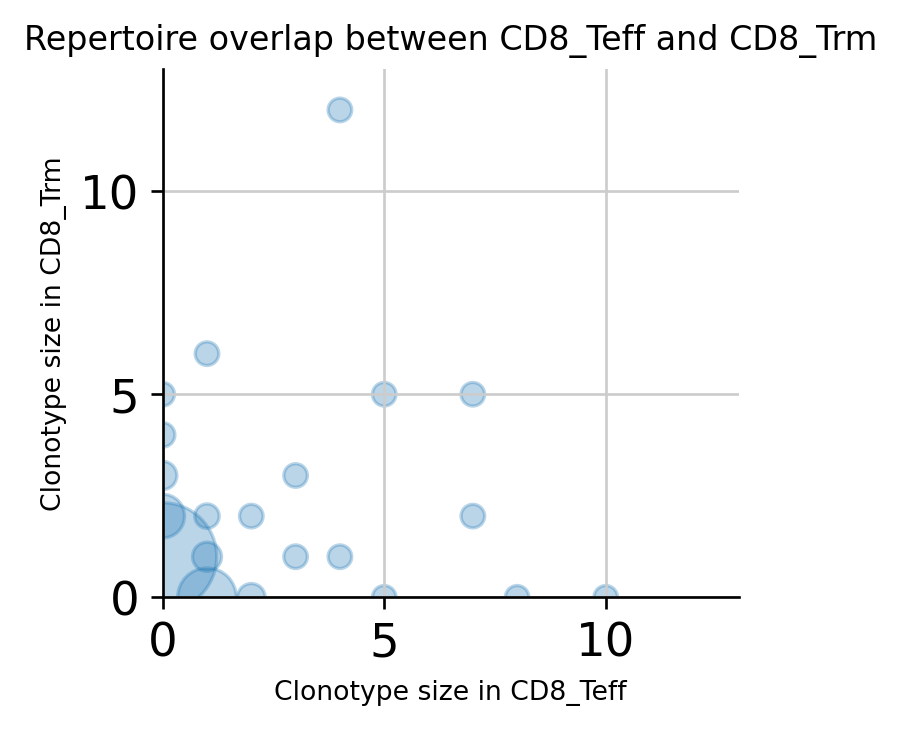
Repertoire overlap of cell types
Just like comparing repertoire overlap among samples, Scirpy also offers comparison between gene expression clusters or cell subpopulations. As an example, repertoire overlap of the two cell types compared above is shown.
[59]:
ir.tl.repertoire_overlap(adata, "cluster")
ir.pl.repertoire_overlap(
    adata, "cluster", pair_to_plot=["CD8_Teff", "CD8_Trm"], fig_kws={"dpi": 120}
)
No handles with labels found to put in legend.
[59]:
<AxesSubplot:title={'center':'Repertoire overlap between CD8_Teff and CD8_Trm'}, xlabel='Clonotype size in CD8_Teff', ylabel='Clonotype size in CD8_Trm'>
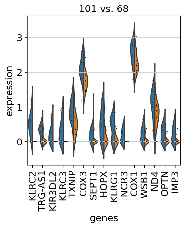
Marker genes in top clonotypes
Gene expression of cells belonging to individual clonotypes can also be compared using Scanpy. As an example, differential gene expression of two clonotypes, found to be specific to cell type clusters can also be analysed.
[60]:
sc.tl.rank_genes_groups(
    adata, "clone_id", groups=["101"], reference="68", method="wilcoxon"
)
sc.pl.rank_genes_groups_violin(adata, groups="101", n_genes=15)
ranking genes
    finished (0:00:00)