A new plotting backend for Scanpy: HoloViews
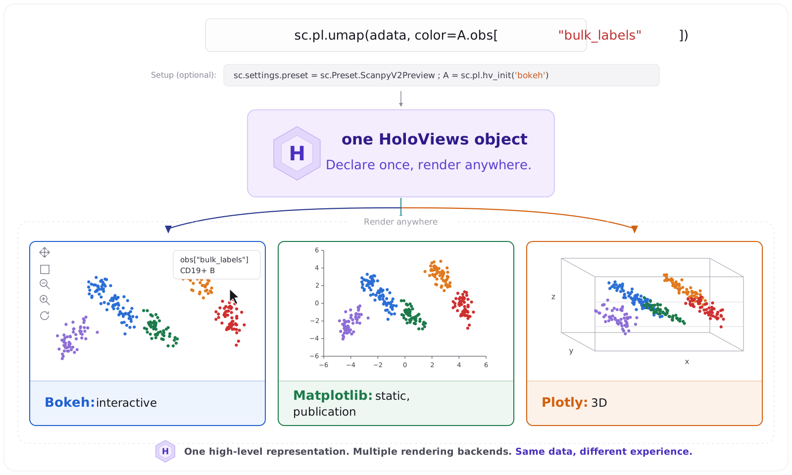
Scanpy’s plotting API has served the single-cell community well for years. But datasets have outgrown static images.
We routinely work with hundreds of thousands, sometimes millions, of cells, and the questions we ask are increasingly interactive: which cells are those, what’s the expression of this gene here, how do these two embeddings line up? Answering them, and more, with a static PNG means re-running a cell, tweaking a parameter, and re-running again.
So we’ve been rebuilding sc.pl on a new foundation: HoloViews.
It’s available today as an opt-in preview, and we’d love your feedback while it’s still taking shape.
What is HoloViews?
HoloViews is part of the HoloViz family of open-source Python visualization tools, alongside Panel, Datashader, and hvPlot. Its central design principle is that the declaration of your data is independent from how it’s plotted.
A HoloViews object is an annotated data container that knows how to render itself. You describe what to show (the x and y dimensions, the value to color by), and HoloViews handles how to draw it. Because the object carries its data, you can inspect it, slice it, compose it, and switch rendering backends without touching your analysis code.
The same object renders through three backends, which means you can write the plot once and pick the one that best fits the moment:
- Bokeh for interactive plots in the browser: pan, zoom, hover, and select.
- Matplotlib for publication-quality static figures.
- Plotly for interactive 3D.
How it fits Scanpy and scverse
HoloViews can be taught to speak AnnData natively.
A small companion package, hv-anndata, gives HoloViews a first-class AnnData interface and the A accessor for pointing at any part of your object.
Most of the time you use the sc.pl shortcuts:
import scanpy as sc

sc.settings.preset = sc.Preset.ScanpyV2Preview
A = sc.pl.hv_init("bokeh")

adata = sc.datasets.pbmc68k_reduced()
sc.pl.umap(adata, color=A.obs["bulk_labels"])
That one line expands to plain HoloViews, where full control lives:
import holoviews as hv

hv.Scatter(
    adata,
    A.obsm["umap"][0],
    [A.obsm["umap"][1], A.obs["bulk_labels"]],
).opts(color=A.obs["bulk_labels"], aspect="square", legend_position="right")
You can drop to this level whenever the shortcut doesn’t expose what you need.
.opts() passes straight through to the backend: there is no bespoke styling buried inside a scanpy function.
There’s no copying columns into a tidy DataFrame, reindexing, or bookkeeping to keep colors aligned with cells.
You reference A.obsm["umap"], A.obs["bulk_labels"], or A.X[:, "GENE"] directly, and hv-anndata handles the plumbing.
The AnnData object stays the single source of truth, in line with the scverse philosophy of organizing workflows around a shared, interoperable data structure.
On top of the interface, hv-anndata ships single-cell-aware components: a ManifoldMap for embeddings, a Dotmap, and a ClusterMap.
The sc.pl plotting functions (scatter, umap, heatmap, violin, stacked_violin, matrixplot, tracksplot, and more) are in Scanpy from 1.13.0a1 onward, available once you set the ScanpyV2Preview preset; each function’s docs page has New and Legacy tabs for both backends.
Because scanpy’s own tools return tidy data, they compose straight into HoloViews.
sc.pl.dotplot, for example, aggregates once with sc.get.aggregate and maps the result onto a HoloViews Points element, with mean expression as color and the fraction of expressing cells as dot size:
markers = ["C1QA", "PSAP", "CD79A", "CD79B", "CST3", "LYZ"]
sc.pl.dotplot(adata[:, markers], A.obs["bulk_labels"])
The whole plot type collapses to an aggregation feeding a data-first element, with no bespoke drawing code: the implementation is only around twenty lines, where the matplotlib version ran to hundreds of lines across several files.
Features we’re excited about
- Full control through
.opts(). You’re no longer limited to the parameters we chose to expose; the full Bokeh, Matplotlib, and Plotly option sets are available, with styling kept out of scanpy’s internals. You declare what to plot throughAand set appearance in.opts(), so the two are easy to tell apart. - Interactivity for free.
With Bokeh, mouse over a cell in a UMAP to read its cluster, gene expression, or any
obsfield with no re-running. - Scales to millions of cells.
Datashader rasterizes the points into a faithful image and re-renders as you zoom, and turning it on can be as simple as
datashade=True. - Composable.
Overlay with
*, lay out side by side with+, and add a marginal histogram with.hist(), soscatter * centroids + expression_violinreplaces a page of axes management. - Existing plots are covered. There’s an equivalent for most of the matplotlib functions you rely on.
Linked brushing
Select a group of cells in a UMAP and watch them highlight in a dotplot or a second embedding; the plots share one selection.
hv-anndata wires this up between its ManifoldMap and Dotmap using HoloViews’ link_selections:
import holoviews as hv
import panel as pn
import hv_anndata

ls = hv.link_selections.instance()
mm = hv_anndata.ManifoldMap(adata=adata, reduction="X_umap", ls=ls)

marker_genes = {"B cells": ["CD79A", "CD79B"], "Monocytes": ["LYZ", "CST3"]}
dm = hv_anndata.dotmap_from_manifoldmap(mm, marker_genes=marker_genes, groupby="bulk_labels")

pn.Column(mm, dm)

# Pull the selected cells back into your workflow. Two documented HoloViews routes:
#   - ls.filter(<element>) filters the source data down to the selection.
#   - Selection1D(source=<plot>).index gives the selected row indices, then adata[index] is the subset.
Try it
The new backend is an opt-in preview.
The legacy matplotlib path and the new HoloViews one live behind the same sc.pl functions, so one setting chooses which is active:
import scanpy as sc

sc.settings.preset = sc.Preset.ScanpyV2Preview  # opt in; default stays on matplotlib
A = sc.pl.hv_init("bokeh")

adata = sc.datasets.pbmc68k_reduced()
sc.pl.scatter(adata, A.X[:, ["PSAP", "C1QA"]], color=A.obs["bulk_labels"]).opts(
    cmap="tab10", show_legend=False
)
By default the preset stays on matplotlib so nothing changes for existing code until you opt in. Matplotlib also stays available indefinitely through the new API, which has multiple backends. This is an early preview and the API will keep changing so the 2.0 version will differ from what you see today. Report bugs, run it on your own data, and tell us what’s missing!
Find us on GitHub, Zulip, and Discourse. Issues, ideas, and pull requests are all welcome.
— Muskan Hashim, Philipp Angerer, and the scverse team.